On aspects of statistical modelling
Shrinkage methods

Ioannis Kosmidis

Professor of Statistics
Department of Statistics, University of Warwick

ioannis.kosmidis@warwick.ac.uk
ikosmidis.com   ikosmidis ikosmidis_

11 April 2025

Outline

• Housekeeping
• Why shrink?
• Ridge regression
• Best subsets
• Lasso regression

Housekeeping

Lectures

There will be 12 hours of lectures in this short course, as follows

Day	Times
Wed	12:00 - 15:00
Thu	10:00 - 13:00
Fri	12:00 - 15:00
Sat	09:00 - 12:00

Footnotes

Some slides have footnotes like¹.

Footnotes have content that should not distract you as you skim through the slides but it is nevertheless important, including:

• Citations
• Commentary
• Exercises

1. this one.

Preliminary material and slide decks

The preliminary material for this short course is at

• Preliminary material

The slide decks for this short course are

• Model selection

• Shrinkage methods 👀

• Beyond generalized linear models

• Nonliner models

• Latent variables

Code-chunks

The R code reproducing the analyses and simulations presented on the slide deck is all embedded on the slides. Just click “[R Code]” wherever it appears.

For example,

library("surreal")
cols <- hcl.colors(4)
set.seed(123)
df <- surreal_text("Shrinkage")
mod <- lm(y ~ ., data = df)
plot(fitted(mod), residuals(mod), xlab = expression(hat(y)), ylab = expression(y - hat(y)),
     pch = 21, bg = cols[3])

From this point onward, when evaluating a code chunk, it is assumed that all previous chunks have been successfully evaluated.

R packages

The code on the slides rely on R version 4.4.2 (2024-10-31) and the packages

package	version
dplyr	1.1.4
ggplot2	3.5.1
ISLR2	1.3-2
glmnet	4.1-8

You can load them (and install them if you do not have them already) by doing

pkgs <- c("ggplot2", "dplyr", "ISLR2", "glmnet")
for (pkg in pkgs)
    if (!require(pkg, character.only = TRUE))
        install.packages(pkg)

Why shrink?

Using all available covariates

Fitting a regression model on all available covariates may result in issues with both prediction accuracy and model interpretability.

e.g. For linear models and least squares

Prediction accuracy

Setting	Least squares results in	Generalizability
\(n >> p\)	low bias and low variance	acceptable out-of sample prediction performance
\(n > p\) but \(n \sim p\)	high-variance and overfitting	poor out-of-sample performance
\(n < p\)	no unique estimators	infinite variance

Interpretability

Including irrelevant variables complicates model interpretation.

It is unlikely to have least squares estimate that are exactly zero.

Singular value decomposition¹

If \(X\) is an \(n \times p\) real matrix, then² \[ X = U \Sigma V^T \]

• \(U\) is an \(n \times n\) orthogonal matrix (\(U^T = U^{-1}\))
• \(V\) is a \(p \times p\) orthogonal matrix
• \(\Sigma = \begin{bmatrix} \Sigma_1 \\ 0_{(n - p) \times p} \end{bmatrix}\), where \(\Sigma_1 = \text{diag}(\sigma_1, \dots, \sigma_p)\) with \(\sigma_1 \geq \dots \geq \sigma_p\)
• \(0_{s \times t}\) is a \(s \times t\) matrix of zeros

1. see, Mandel (1982) for an instructive paper on SVD and its use in regression, with particular focus on (near) collinearity and its implications

2. From Gander et al. (2014, sec. 6.3): “With the SVD one x-rays a matrix”.

Sensitivity of least squares on \(X\)

The sum of squared errors can be written as \[ \|Y - X\beta\|_2^2 = \|U^T Y - U^T X V V^T \beta\|_2^2 = \|U^T Y - \Sigma \beta^*\|_2^2 \]

which expands to \[ \sum_{j = 1}^p (u_j^T Y - \sigma_j \beta_j^*)^2 + \sum_{j = p+1}^n(u_j^T Y)^2 \]

The least squares estimate can then be written as \[ \hat{\beta} = \sum_{j = 1}^p \frac{1}{\sigma_j} v_j u_j^T Y \] \(\hat\beta\) is sensitive to the magnitude of the singular values of \(X\); instabilities are to be expected when singular values are small.

Sensitivity of Least Squares on \(X\)

\(X\)

(X <- matrix(c(1, 0, 0, 0, 1e-06, 0), 3, 2))

     [,1]  [,2]
[1,]    1 0e+00
[2,]    0 1e-06
[3,]    0 0e+00

\(Y\)

(Y <- c(1, 0, 1))

[1] 1 0 1

A “small” perturbation to \(X\)

(dX <- matrix(c(0, 0, 0, 0, 0, 1e-08), 3, 2))

     [,1]  [,2]
[1,]    0 0e+00
[2,]    0 0e+00
[3,]    0 1e-08

Y ~ -1 + X

coef(summary(lm(Y ~ -1 + X)))

   Estimate Std. Error t value Pr(>|t|)
X1        1      1e+00       1      0.5
X2        0      1e+06       0      1.0

Y ~ -1 + I(X + dX)

coef(summary(lm(Y ~ -1 + I(X + dX))))

           Estimate Std. Error t value  Pr(>|t|)
I(X + dX)1        1 9.9995e-01 1.00005 0.4999841
I(X + dX)2     9999 9.9990e+05 0.01000 0.9936340

SVD of \(X\)

svd(X, nu = nrow(X))

$d
[1] 1e+00 1e-06

$u
     [,1] [,2] [,3]
[1,]    1    0    0
[2,]    0    1    0
[3,]    0    0    1

$v
     [,1] [,2]
[1,]    1    0
[2,]    0    1

SVD of \(X + dX\)

svd(X + dX, nu = nrow(X))

$d
[1] 1.00000e+00 1.00005e-06

$u
     [,1]       [,2]       [,3]
[1,]    1  0.0000000  0.0000000
[2,]    0 -0.9999500 -0.0099995
[3,]    0 -0.0099995  0.9999500

$v
     [,1] [,2]
[1,]    1    0
[2,]    0   -1

Collinearity

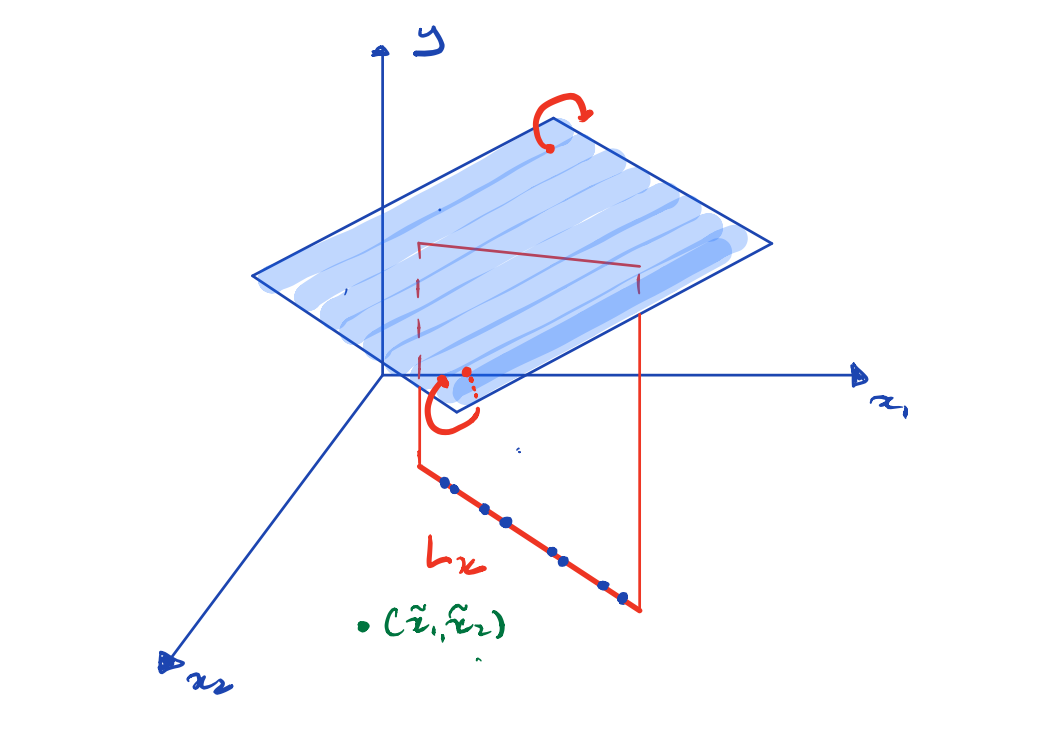
Prediction at a new point \((\tilde{x}_1, \tilde{x}_2)^\top\) is not unique unless it lies on \(L_x\)

Bias-variance tradeoff and prediction accuracy

Gauss-Markov theorem

The Gauss-Markov theorem¹ implies that the least-squares estimator has the smallest mean squared error amongst all linear unbiased estimators

Prediction accuracy

Consider the prediction \(\tilde{Y} = \tilde{x}^\top\beta + \epsilon_0\) of a new response at covariate setting \(\tilde{x}\).

Under the Normal linear model the expected prediction error of a prediction \(\tilde{x}^\top\hat\beta\) is \[ \sigma^2 + \tilde{x}^\top\underbrace{\mathop{\mathrm{E}}\left\{(\hat\beta - \beta)^\top(\hat\beta - \beta)\right\}}_{\text{Mean squared error}} \tilde{x} \]

Can we trade some bias for a reduction in variance, and better mean squared error?

1. see e.g. https://en.wikipedia.org/wiki/Gauss–Markov_theorem}

\(p > n\)

When \(p > n\), \(X\) does not have full column rank and the least squares problem does not have a unique solution.

Best subsets and stepwise regression

Computational Efficiency

Best subset selection is combinatorially expensive for general models.

Stability

Stepwise regression and best subset selection may suffer from high variance, leading to unstable model selection.

Collinearity

Stepwise methods can behave unpredictably in the face of collinearity.

Overfitting

Stepwise methods rely on local data-dependent decisions after seeing a sequence of models, which can lead to overfitting.

\(\ell_q\) balls \(\{\beta \in \Re^3 \mid |\beta_1|^q + |\beta_2|^q + |\beta_3|^q \le m\}\)

\(q = 2\)

\(q = 3\)

\(q = 4\)

Ridge regression

Ridge regression and linear models

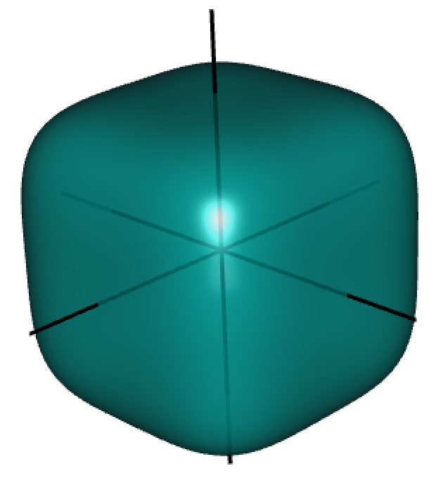
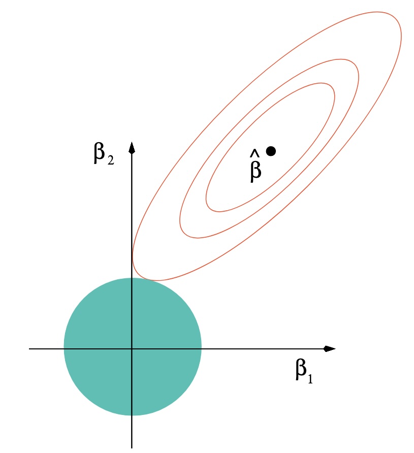
For \(\lambda > 0\), the ridge estimator of \(\beta\) is \[ \begin{aligned} \hat\beta_\lambda & = \arg \min_{\beta} \|Y - X\beta \|^2_2 + \underbrace{\lambda \|\beta \|^2_2}_{\text{ridge penalty}} \\ \notag & = (X^\top X + \lambda {I}_p)^{-1} X^\top Y \end{aligned} \tag{1}\] where \({I}_p\) is the \(p \times p\) identity matrix^{1 2}

(1) is a convex optimisation problem (the objective is the sum of two convex functions of \(\beta\)) and has always a unique solution.

Ridge regression adds a multiple of a full-rank matrix (!) to \(X^\top X\), which stabilizes inversion when the columns of \(X\) are (nearly) dependent.

1. See Hoerl & Kennard (1970) for the proposal of ridge regression

2. Exercise: derive the closed form expression for \(\hat\beta_\lambda\).

\(X\) matrix

Typically, we take \(X\) having no intercept column, and consisting of centered explanatory variables (\(x_{ij} = x_{ij}^{(o)} - \sum_{i = 1}^n{x_{ij}^{(o)}}/n\)). Ridge estimation can happen in two steps¹

1. Compute \(\hat\beta_\lambda\) as in (1)

2. Estimate the intercept as \(\hat\beta_0 = \bar{y} - \sum_{j = 1}^p \bar{v}_j \hat{\beta}_{\lambda,j}\), where \(v_j\) here is the \(j\)th column of \(X\).

Ridge regression is not invariant to scaling of the explanatory variables so we generally ensure that \(X\) has standardised columns.

1. Exercice: Consider the model \(Y = \beta_0 {1} + X \beta + \epsilon\) where \(X\) has centered columns. Show that the two step process results in the ridge regression estimator for \(\beta_0\) and \(\beta_\lambda\) when \(\beta_0\) is not in the penalty.

Shrinkage

Directly from (1), the ridge estimates will converge to zero as \(\lambda \to \infty\) regardless of the data

Hastie et al. (2015, fig. 2.2)

In terms of the SVD of \(X\) \[ \begin{aligned} \hat\beta_\lambda = \sum_{j = 1}^p \frac{\sigma_j}{\sigma_j^2 + \lambda} v_j u_j^T Y \end{aligned} \]

e.g. \(X\) with orthogonal columns (\(X^\top X = {I}_p\)) \[ \begin{aligned} \hat\beta_\lambda & = (X^\top X + \lambda {I}_p)^{-1} X^\top Y \\ & = (1 + \lambda)^{-1} (X^\top X)^{-1} X^\top Y = (1 + \lambda)^{-1} \hat\beta \end{aligned} \]

The ridge estimator scales the least squares one by a factor and \(|\hat\beta_{\lambda_2}| < |\hat\beta_{\lambda_1}|\) for \(\lambda_1 < \lambda_2\) (element-wise “\(<\)” and “\(|.|\)” here).

Shrinkage

In terms of fitted values, using the SVD of \(X\)

Least squares

\[ X \hat\beta = \sum_{j = 1}^p u_j u_j^\top Y \] (well-defined even when \(n < p\))

Ridge regression

\[ X \hat\beta_\lambda = \sum_{j = 1}^p \frac{\sigma_j^2}{\sigma_j^2 + \lambda} u_j u_j^\top Y \]

Ridge shrinks more along the principal component directions \(u_j\) that correspond to low variance (small \(\sigma_j\)), and less along the directions \(u_j\) that correspond to high variance.

Variable selection (sort of)

Ridge regression shrinks coefficients towards zero, adaptively depending on the size of the singular values of \(X\). However, it does not set them exactly to zero.

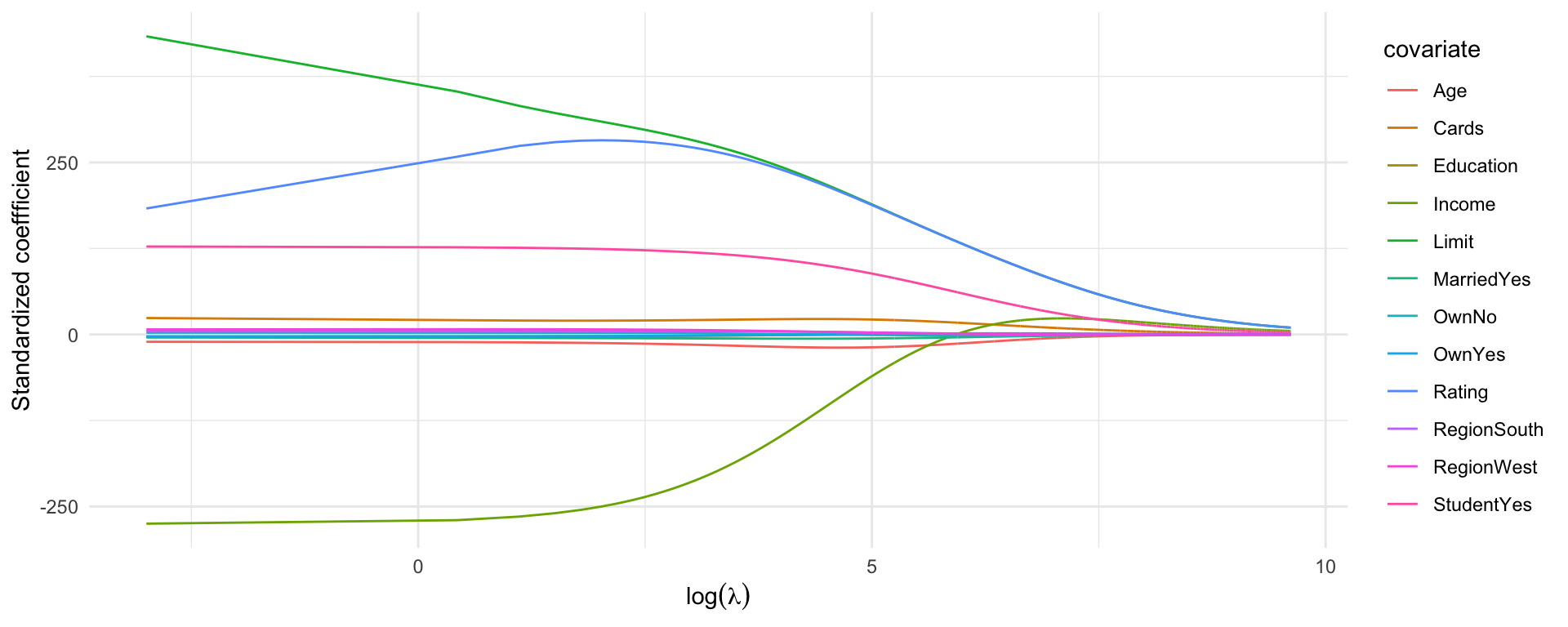
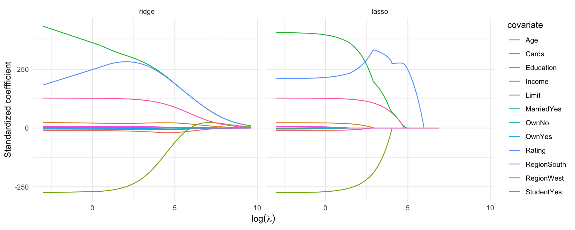
Solution path

The set of all ridge regression estimates \(\{\hat\beta_\lambda: \lambda > 0\}\) is called the solution path.
e.g. using MASS::lm.ridge() for ISLR2::Credit, which uses an SVD of \(X\) to get the whole solution path (if you can compute it)

library("MASS")
data("Credit", package = "ISLR2")
fm <- Balance ~ -1 + .
credit_mf <- model.frame(fm, data = Credit)
X <- model.matrix(fm, credit_mf)
X_scaled <- scale(X)
Y <- scale(model.response(credit_mf), scale = FALSE)
grid_size <- 10000
lambda_grid <- seq(15000, 0.05, length = grid_size)
ridge_fit <- lm.ridge(Y ~ -1 + X_scaled, lambda = lambda_grid)
## Using glmnet
## ridge_fit <- glmnet(X_scaled, Y, alpha = 0, lambda = lambda_grid)
## plot(ridge_fit, xvar = "lambda", label = TRUE, main = "Ridge solution path",
##      ylab = "Standardized coefficients")
df_ridge <- data.frame(lambda = rep(lambda_grid, ncol(X)),
                 covariate = rep(colnames(X), each = grid_size),
                 estimate = c(coef(ridge_fit)),
                 method = "ridge")
ggplot(df_ridge) +
    geom_line(aes(x = log(lambda), y = estimate, col = covariate)) +
    theme_minimal() +
    labs(x = expression(log(lambda)), y = "Standardized coeffficient")

Ridge regression retains all features but reduces their impact as \(\lambda\) increases.

Bias and variance

Expectation of \(\hat\beta_\lambda\)

\[ \mathop{\mathrm{E}}(\hat\beta_\lambda) = X^\top X(X^\top X + \lambda {I}_p)^{-1}\beta \]

The ridge estimator is biased even when \(\hat\beta\) is not.

Variance of \(\hat\beta_\lambda\)

\[ \mathop{\mathrm{var}}(\hat\beta_\lambda) = \sigma^2(X^\top X + \lambda {I}_p)^{-1}X^\top X (X^\top X + \lambda {I}_p)^{-1} \]

The variance of \(\hat\beta_\lambda\) goes to zero as \(\lambda \to \infty\).

Also, \(\mathop{\mathrm{var}}(\hat\beta_\lambda) - \mathop{\mathrm{var}}(\hat\beta)\) is a non-negative definite matrix. In that sense, the distribution of \(\hat\beta_\lambda\) under the linear model is more concentrated around its expectation than that of \(\hat\beta\).

Bias-variance tradeoff

There exists \(\lambda^* > 0\) such that \[ \mathop{\mathrm{E}}\left\{ (\hat\beta - \beta)(\hat\beta - \beta)^\top \right\} - \mathop{\mathrm{E}}\left\{ (\hat\beta_\lambda - \beta)(\hat\beta_\lambda - \beta)^\top \right\} \] is positive definite whenever \(0 < \lambda < \lambda^*\).^{1 2}

1. See Theobald (1974, Theorem 2).

2. Exercise: Derive \(M_\lambda = \mathop{\mathrm{E}}\left\{ (\hat\beta_\lambda - \beta)(\hat\beta_\lambda - \beta)^\top \right\}\) for \(X\) with orthogonal columns (\(X^\top X = {I}_p\), \(n > p\)), find its minimum with respect to \(\lambda\), and compare it with \(M_0\).

Degrees of freedom and choice of \(\lambda\)

Degrees of freedom and generalized cross-validation criterion

We can write \(X\hat\beta_\lambda = H(\lambda)Y\). The effective degrees of freedom for ridge regression are then¹ \[ \mathop{\mathrm{tr}}\left\{H(\lambda)\right\} = \sum_{i = 1}^p \frac{\sigma_i^2}{\sigma_i^2 + \lambda} \le p \] where \(\sigma_i\) is the \(i\)th singular value of \(X\). Then, the generalized cross-validation criterion is \[ \frac{1}{n} \sum_{i = 1}^n \left[ \frac{y_i - x_i^\top\hat\beta_\lambda}{1 - \mathop{\mathrm{tr}}{\left\{H(\lambda)\right\}/n}}\right]^2 \]

Choice of \(\lambda\)

Choose \(\lambda\) that minimises the generalised cross-validation criterion.²

1. Exercise: Show this.

2. Cross-validated MSE, and AIC/BIC with \(\mathop{\mathrm{tr}}\left\{H(\lambda)\right\}\) degrees of freedom can also be used. Patil et al. (2021) show that both leave-one-out cross-validation and generalized cross validation are asymptotically equivalent to using the oracle out-of-sample prediction error.

Efficient ridge regression for \(p>>n\)

\[ \hat\beta_\lambda = (\underbrace{X^\top X + \lambda {I}_p}_{p \times p})^{-1} X^\top Y \]

If \(p >> n\) then inverting the \(p \times p\) matrix can be particularly demanding. Actually, in such cases the computational cost for \(\hat\beta_\lambda\) is \(O(p^3)\)

Efficient ridge regression for \(p>>n\)

It can be shown¹ that \[ \hat\beta_\lambda = V_1 (\underbrace{\lambda {I}_n + R^\top R}_{n \times n})^{-1} R^\top Y \tag{2}\] where \(R\) (\(n \times n\)) and \(V_1\) (\(p \times n\)) such that \(X = R V_1^\top\) with \(V_1^\top V_1 = I_n\) (SVD tells us that we can always write \(X\) this way).²

This re-expression reduces the computational cost to \(O(n p^2)\) which is considerably faster than \(O(p^3)\) for \(p >> n\).

1. see Hastie & Tibshirani (2004)

2. Exercise: Attempt to show (2); the key ingredient is the Sherman-Morrison-Woodbury identity.

\(\ell_q\) balls \(\{\beta \in \Re^3 \mid |\beta_1|^q + |\beta_2|^q + |\beta_3|^q \le m\}\)

\(q = 2\)

\(q = 3\)

\(q = 4\)

\(q = 1\)

\(q = 3/4\)

\(q = 1/2\)

Best subsets

Best subsets and linear models

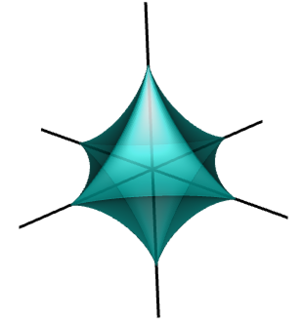
For \(\lambda > 0\), the lagrangian version of best subsets is \[ \begin{aligned} \beta_\lambda^\dagger & = \arg \min_{\beta} \|Y - X\beta \|^2_2 + \underbrace{\lambda \|\beta \|_0}_{\text{$\ell_0$ penalty}} \end{aligned} \tag{3}\]

This is a non-convex problem.

Oracle least squares in sparse linear models

Suppose that \(Y = X \beta^* + \epsilon\) with \(\epsilon \sim N(0, \sigma^2 I_n)\) and let \(S = \{j \in \mathcal{I} \mid \beta_{j}^* \ne 0 \}\) be the true active set.

Then, the oracle least squares estimator \(\hat\beta^{(oracle)}\) has its elements zero, except those indexed in \(S\), which are set to \((X_{[S]}^\top X_{[S]})^{-1} X_{[S]}^\top Y\).

It can be shown that, for fixed \(X\), the prediction risk of the oracle least squares estimator is \[ \frac{1}{n} \mathop{\mathrm{E}}\|X(\hat\beta^{(oracle)} - \beta_0) \|_2^2 = \sigma^2 \frac{|S|}{n} \]

Best subsets in sparse linear models

For fixed \(X\), and \(\lambda \asymp \sigma^2\log d\), the best subset selection estimator satisfies \[ \frac{\mathop{\mathrm{E}}\|X(\beta^\dagger - \beta^*)\|_2^2 / n}{\sigma^2 |S| / n} \leq 4\log p + 2 + o(1), \quad \text{as $n,p \to \infty$}. \] without any conditions on the predictor matrix \(X\). Moreover, \[ \inf_{\hat\beta} \, \sup_{X,\beta^*} \, \frac{\mathop{\mathrm{E}}\|X(\hat\beta- \beta^*)\|_2^2/n}{\sigma^2 |S|/n} \geq 2 \log p - o(\log p) \] where the infimum is over all estimators \(\hat\beta\), and the supremum is over all predictor matrices \(X\) and underlying coefficients \(\beta^*\) that have \(\ell_0\)-sparsity equal at most \(|S|\).¹

Best subset selection is optimal in terms of rate as it achieves the optimal risk inflation over the risk of the oracle least squares estimator.

1. See Foster & George (1994) for proof.

Lasso regression

Lasso regression and linear models

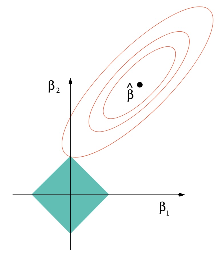
For \(\lambda > 0\), the Lasso (Least Absolute Selection and Shrinkage Operator) estimator of \(\beta\) is \[ \begin{aligned} \tilde\beta_\lambda & = \arg \min_{\beta} \frac{1}{2n}\|Y - X\beta \|^2_2 + \underbrace{\lambda \|\beta \|_1}_{\text{Lasso penalty}} \end{aligned} \tag{4}\]

(4) is a convex optimisation problem (the objective is the sum of two convex functions of \(\beta\)) but does not always have a unique solution¹. What is always unique are the fitted values \(X \tilde{\beta}_\lambda\).

When the columns of \(X\) are in general position², then the Lasso solutions are unique.

If the elements of the model matrix \(X\) are drawn from a continuous probability distribution, then with probability one the data are in general position.

Non-uniqueness of the Lasso solutions can occurs with discrete-valued data, such as those arising from dummy variables for categorical predictors.³

1. The \(1/(2n)\) factor can be omitted here; it is just convenient when deriving estimation algorithms and the scaling of \(\lambda\) in theoretical results.

2. The columns of \(X\), \(v_1, \ldots, v_p\), are in general position if any affine subspace \(L \subset \Re^n\) of dimension \(k < n\) contains at most \(k + 1\) elements of the set ${v_1, , v_p} excluding antipodal pairs of points (that is, points differing only by a sign flip

3. See Tibshirani (2013) for uniqueness proof under general position and discussion.

\(X\) matrix

Typically, we take \(X\) having no intercept column, and consisting of centered explanatory variables (\(x_{ij} = x_{ij}^{(o)} - \sum_{i = 1}^n{x_{ij}^{(o)}}/n\)). Lasso estimation can happen in two steps

1. Compute \(\tilde\beta_\lambda\) as in (4)

2. Estimate the intercept as \(\tilde\beta_0 = \bar{y} - \sum_{j = 1}^p \bar{v}_j \tilde{\beta}_{\lambda,j}\), where \(v_j\) here is the \(j\)th column of \(X\)

Like ridge, Lasso regression is not invariant to scaling of the explanatory variables so we generally ensure that \(X\) has standardised columns.

Shrinkage

e.g. using glmnet::glmnet() for ISLR2::Credit

library("MASS")
data("Credit", package = "ISLR2")
fm <- Balance ~ -1 + .
credit_mf <- model.frame(fm, data = Credit)
X <- model.matrix(fm, credit_mf)
X_scaled <- scale(X)
Y <- scale(model.response(credit_mf), scale = FALSE)
grid_size <- 10000
lambda_grid <- seq(1000, 0.05, length = grid_size)
lasso_fit <- glmnet(X_scaled, Y, alpha = 1, lambda = lambda_grid, intercept = FALSE)
df_lasso <- data.frame(lambda = rep(lambda_grid, ncol(X)),
                       covariate = rep(colnames(X), each = grid_size),
                       estimate = c(t(as.matrix(coef(lasso_fit)[-1, ]))),
                       method = "lasso")
ggplot(rbind(df_lasso, df_ridge) |>
       mutate(method = factor(method, levels = c("ridge", "lasso"), ordered = TRUE))) +
    geom_line(aes(x = log(lambda), y = estimate, col = covariate)) +
    theme_minimal() +
    facet_grid(~ method) +
    labs(x = expression(log(lambda)), y = "Standardized coeffficient")

For large enough \(\lambda\), Lasso will shrink all the coefficients to exactly zero.

Shrinkage

Hastie et al. (2015, fig. 2.2)

Hastie et al. (2015, fig. 2.2)

Computing the Lasso fit

Cyclic coordinate descent

One particularly elegant way to find the solution of (4) is via cyclic coordinate descent, where the update

\[ \tilde{\beta}_{\lambda, j} = \mathcal{S}_\lambda\left(\frac{1}{n} v_j^\top r^{(j)}\right) \tag{5}\]

is applied repeatedly in a cyclical manner until the coefficients do not change substantially.

In (5), \(S_\lambda(x) = {\rm sign}(x) \max\{|x| - \lambda, 0\}\) is the soft-thresholding operator, \(v_j\) is \(j\)th column of \(X\), \(r_{i}^{(j)} = y_i - \sum_{k \ne j} x_{ij} \tilde{\beta}_{\lambda, k}\) is the partial residual.

Pathwise coordinate descent

Typically, we compute the solution path using “warm starts”, i.e. we start with a large enough \(\lambda\) so that the only solution is the zero vector, decrease \(\lambda\) and run coordinate descent, decrease again using the previous solution as starting values, and so on.¹

1. See Hastie et al. (2015) for other methods to compute the lasso solution.

Degrees of freedom and choice of \(\lambda\)

Choosing predictors based on the response (e.g., forward stepwise selection) tends to use more than \(p\) degrees of freedom.

Lasso selects covariates like forward stepwise regression but also shrinks coefficients.

For fixed \(\lambda\) the shrinkage effect reduces degrees of freedom to exactly the number of non-zero parameters, counteracting the inflation caused by adaptive selection.¹

Choice of \(\lambda\)

Choose \(\lambda\) that minimizes cross-validated MSE.²

1. See Tibshirani & Taylor (2012) for the degrees of freedom of the Lasso.

2. Chetverikov et al. (2021) derive error bounds for the Lasso estimator when the tuning parameter is chosen using \(k\)-fold cross-validation.

Lasso in linear models: Prediction error

Suppose that \(Y = X \beta^* + \epsilon\) with \(\epsilon \sim N(0, \sigma^2 I_n)\) for some \(\beta^* \in \Re^p\).¹

Slow rate

If \(\|\beta^*\|_1 \le R_1\) and \(\lambda = c \sigma \sqrt{\log p / n}\) for \(R_1, c > 0\), then there exists \(c_1 > 0\) such that with high probability, a solution to (4) satisfies \[ \frac{1}{n} \|X(\tilde\beta_\lambda - \beta^*)\|_2^2 \le c_1 \sigma R_1 \sqrt{\frac{\log p}{n}} \]

Fast rate

Let \(S = \{j \in \mathcal{I} \mid \beta_{j}^* \ne 0 \}\). If \(\|X \nu\|_2^2 / n \ge \gamma \|\nu\|_2^2\) for all nonzero \(\nu \in \Re^p\) with \(\|\nu_{[\mathcal{I} \setminus J]}\|_1 \le 3\|\nu_{[J]}\|_1\) for \(\gamma > 0\) and for all subsets \(J \subseteq \mathcal{I}\) with \(|J| = |S|\) (restricted eigenvalue condition), then for \(\lambda = c \sigma \sqrt{\log p / n}\) with \(c > 0\), there exists \(c_2 > 0\) such that with high probability, (4) satisfies \[ \frac{1}{n} \|X(\tilde\beta_\lambda - \beta^*)\|_2^2 \le c_2 \frac{\sigma^2}{\gamma} \frac{|S|\log p}{n} \]

1. For a detailed and precise treatment of theoretical results (e.g. consistency, prediction quality, and variable selection properties) for the Lasso see Hastie et al. (2015, sec. 11) and Wainwright (2019, sec. 7).

Lasso in linear models: Variable selection consistency

Suppose that \(Y = X \beta^* + \epsilon\) with \(\epsilon \sim N(0, \sigma^2 I_n)\) for some \(\beta^* \in \Re^p\), and that \(S = \{j \in \mathcal{I} \mid \beta_{j}^* \ne 0 \}\) is the true active set.

Also assume that the following assumptions hold:

• The smallest eigenvalue of \(X_{[S]}^\top X_{[S]} / n\) is bounded below by \(C > 0\)

• There exists \(a \in [0,1]\) such that \(\max_{j \in \mathcal{I} \setminus S} \|(X_{[S]}^\top X_{[S]})^{-1} X_{[S]} v_j \|_1 \le 1 - \alpha\) (mutual incoherence / irrepresentability), where \(v_j\) is the \(j\)th column of \(X\)

• \(\max_{j \in \mathcal{I}} \|v_j\|_2 / \sqrt{n} \le K\)

Lasso in linear models: Variable selection consistency

Then¹, for \(\lambda \ge 8 K \sigma / \gamma \sqrt{ log p / n}\), with high probability

1. Uniqueness: The solution of (4) is unique

2. No false inclusion: \(S \subseteq \tilde{S} = \{\tilde\beta_j \ne 0 \mid j \in \mathcal{I}\}\)

3. \(\ell_\inf\) bound:

\[ \|\tilde\beta_{\lambda, [S]} - \beta_{[S]}^*\|_\infty \le \overbrace{\lambda \left[ \frac{4 \sigma}{\sqrt{C}} + \|(X_{[S]}^\top X_{[S]} / n)^{-1}\|_\infty \right]}^{B(\lambda, \sigma \,;\,X)} \]

4. No false exclusion: The Lasso solution includes of \(j \in S\) such that \(|\beta_j^*| > B(\lambda, \sigma \,;\,X)\) and hence is variable selection consistent as long as \(\min_{j \in S} |\beta_j^*| > B(\lambda, \sigma \,;\,X)\)

1. See, Hastie et al. (2015, sec. 11.4)

Shrinkage methods

Properties	Best subsets	Ridge	Lasso
Convex problem		✔	✔
Closed form estimates of \(\beta\)	✔	✔
Uniqueness of solution		✔
Collinearity handling		✔
Shrinkage		✔	✔
\(p > n\)	✔	✔	✔
Variable selection	✔		✔

Discussion

There are more theoretical results on the behaviour of Lasso and ridge regression in terms of estimation consistency, prediction quality, and variable selection consistency for a range of asymptotic regimes¹.

The methods, algorithms, and theoretical analyses have also been extended for a wide range of modelling settings², and there is a steady stream of application and corresponding theoretical results in novel settings.

There is also a wide range of penalties in an attempt to address the limitations of ridge and Lasso regression.

1. Wainwright (2019) and Hastie et al. (2015) organize and provide authoritative accounts of such developments

2. e.g. see Hastie et al. (2015, Chapter 3, Section 4.4. and Chapter 9) for \(\ell_1\) penalties for estimation and selection in generalized linear models, generalized additive models, and graphical models, respectively.

Elastic Net

Combination of an \(\ell_1\) (Lasso type) and an \(\ell_2\) (ridge type) penalty

Balances sparsity and collinearity

Useful when predictors are highly correlated

Zou, H., & Hastie, T. (2005). Regularization and variable selection via the elastic net. Journal of the Royal Statistical Society: Series B, 67(2), 301-320.

SCAD and MC+

SCAD (Smoothly Clipped Absolute Deviation) and MC+ (Minimax Concave Penalty):

Address bias in Lasso by using non-convex penalties

Preserve sparsity, and provide unbiased estimation for large coefficients

Fan, J., & Li, R. (2001). Variable selection via nonconcave penalized likelihood and its oracle properties. Journal of the American Statistical Association, 96(456), 1348-1360.

Zhang, C. H. (2010). Nearly unbiased variable selection under minimax concave penalty. The Annals of Statistics, 38(2), 894-942.

Adaptive Lasso

Uses a weighted \(\ell_1\) penalty, varying the strength of penalization across coeffficients

Improves variable selection consistency over Lasso

Reduces bias in coefficient estimation, recovering their consistency under assumptions

Zou, H. (2006). The adaptive Lasso and its oracle properties. Journal of the American Statistical Association, 101(476), 1418-1429.

Square Root Lasso

Penalizes the square root of the sum of squared errors

The tuning parameter that delivers near-oracle performance (a fast rate) does not depend on \(\sigma\)

Belloni, A., Chernozhukov, V., & Wang, L. (2011). Square-root Lasso: pivotal recovery of sparse signals via conic programming. Biometrika, 98(4), 791-806.

Group Lasso

Extends Lasso to grouped variables

Encourages selection of entire groups of related features

Useful when predictors have natural groupings (e.g., categorical variables with multiple levelsm additive regression models, etc.)

Yuan, M., & Lin, Y. (2007). Model selection and estimation in regression with grouped variables. Journal of the Royal Statistical Society: Series B, 68(1), 49-67.

Debiased and thresholded ridge

Takes advantage of the uniqueness of the closed-form solution in ridge regression

Thresholds a debiased ridge estimator to result in a variable selection and estimation methods with similar guarantees to the Lasso

Zhang, Y., & Politis, D. N. (2022). Ridge regression revisited: debiasing, thresholding, and bootstrap. The Annals of Statistics, 50(3), 1401-1422.

References

Chetverikov, D., Liao, Z., & Chernozhukov, V. (2021). On cross-validated Lasso in high dimensions. The Annals of Statistics, 49(3). https://doi.org/10.1214/20-AOS2000

Foster, D. P., & George, E. I. (1994). The risk inflation criterion for multiple regression. The Annals of Statistics, 22(4). https://doi.org/10.1214/aos/1176325766

Gander, W., Gander, M. J., & Kwok, F. (2014). Scientific computing - an introduction using maple and MATLAB. Springer Publishing Company, Incorporated.

Hastie, T., & Tibshirani, R. (2004). Efficient quadratic regularization for expression arrays. Biostatistics, 5(3), 329. https://doi.org/10.1093/biostatistics/kxh010

Hastie, T., Tibshirani, R., & Wainwright, M. (2015). Statistical learning with sparsity: The lasso and generalizations. CRC Press, Taylor & Francis Group.

Hoerl, A. E., & Kennard, R. W. (1970). Ridge regression: Biased estimation for nonorthogonal problems. Technometrics, 12(1), 55–67. http://www.jstor.org/stable/1267351

Mandel, J. (1982). Use of the singular value decomposition in regression analysis. The American Statistician, 36(1), 15–24. http://www.jstor.org/stable/2684086

Patil, P., Wei, Y., Rinaldo, A., & Tibshirani, R. (2021). Uniform consistency of cross-validation estimators for high-dimensional ridge regression. Proceedings of The 24th International Conference on Artificial Intelligence and Statistics, 3178–3186. https://proceedings.mlr.press/v130/patil21a.html

Theobald, C. M. (1974). Generalizations of mean square error applied to ridge regression. Journal of the Royal Statistical Society. Series B (Methodological), 36(1), 103–106. http://www.jstor.org/stable/2984775

Tibshirani, R. J. (2013). The lasso problem and uniqueness. Electronic Journal of Statistics, 7. https://doi.org/10.1214/13-EJS815

Tibshirani, R. J., & Taylor, J. (2012). Degrees of freedom in Lasso problems. The Annals of Statistics, 40(2), 1198–1232. https://www.jstor.org/stable/41713670

Wainwright, M. J. (2019). High-dimensional statistics: A non-asymptotic viewpoint (1st ed.). Cambridge University Press. https://doi.org/10.1017/9781108627771