Accessibility of HTML pages from R Markdown Tweet

Images from external files

The <img> HTML tag has an alt attribute, which is what a screen reader will read when it gets to the image. This is our opportunity to provide some alt text for readers relying on screen readers to access the content. The <img> HTML tag also has a title attribute that is shown as a tooltip when you hover over the image in a browser.

Markdown’s ![A-text](path-to-img-file "B-text") syntax for including images from external files allows for the inclusion of all alt text, title text, and captions. However, depending on whether the image is in a paragraph or whether A-text or B-text are supplied or not, what ends up being the title, caption, and alt text varies. Of course, it varies in an entirely predictable way, but still, it can get hard to remember to break that line or add a \ after the inclusion of an image (at least for me).

R Markdown’s default behaviour, on the other hand, is to use the text for a figure caption, both as a caption and as alt text, which is not ideal in many circumstances.

For those reasons, when I author R Markdown documents I rely on knitr::include_graphics() and the custom knitr hook below that allows me to specify any or all of the title, alt-text and caption.

my_plot_hook <- function(x, options) {
    base <- knitr::opts_knit$get('base.url')
    if (is.null(base)) {
        base <- ""
    }
    alt <- ifelse(is.null(options$alt), "", options$alt)
    cap <- ifelse(is.null(options$caption), "", options$caption)
    tit <- ifelse(is.null(options$title), "", options$title)
    w <- options[['out.width']]
    h <- options[['out.height']]
    if (!is.null(w) | !is.null(h)) {
        str <- paste(c(sprintf('width=%s', w),
                       sprintf('height=%s', h)), collapse = " ")
        str <- paste("{", str, "}")
    }
    if (cap == "") {
        sprintf('![%s](%s%s %s)%s\\', alt, base, x, paste0("'", tit, "'"), str)
    }
    else {
        sprintf('![%s](%s%s %s)%s\\\n\n<blockquote><p class = "caption">%s</p></blockquote>', alt, base, x, paste0("'", tit, "'"), str, cap)
    }
}

The above hook is an extended version of a hook that appeared in a discussion at RStudio’s community forum. It allows us to specify alt text, caption text (within a <blockquote> HTML tag to distinguish it from the standard text) and title text, all using chunk options. Before I continue with a demo, note that the hook is specific to getting HTML output from a single R Markdown file via pandoc. I cannot provide any guarantees of it working as advertised for other output formats or more involved collections of R Markdown files (e.g. bookdown projects). See, for example, knitr’s GitHub repository for how involved the code for the default plot hooks has to be to deliver support for a range of output formats. Also, any other figure- and image-specific chunk options other than title, alt, caption, out.width, and out.height will be ineffective when you are using this hook (but that’s all the options I typically need with HTML content).

Let’s replace the default plot hook with my_plot_hook

library("knitr")
knit_hooks$set(plot = my_plot_hook)

Then, the code chunks

``{r, echo = FALSE}
cap_txt <- "Grey cat. A picture by Thomas Gass downloaded from [Wikimedia](https://commons.wikimedia.org/wiki/Category:Felis_silvestris_catus#/media/File:Greycat.jpg) distributed under [CC BY 2.5](https://creativecommons.org/licenses/by/2.5)."
alt_txt <- "'Misty', female cat, aged around two and a half years."
title_txt <- "A grey cat staring at you."
img_url <- "https://upload.wikimedia.org/wikipedia/commons/1/15/Greycat.jpg"
```

```{r, echo = FALSE, caption = cap_txt, alt = alt_txt, title = title_txt}
knitr::include_graphics(img_url)
```

give

Grey cat. A picture by Thomas Gass downloaded from Wikimedia distributed under CC BY 2.5.

If you hover over the image (but do not to look into the cat’s eyes for too long!) you get a tooltip with the title “A grey cat staring at you”. The caption is the quoted text immediately below the image, and a screen reader will say “Misty, female cat, aged around two and a half years” when the image is selected.

Images generated by code-blocks

We can use the same hook for images that are generated programmatically. For example, suppose that we want to demonstrate the color-blind friendly palettes recommended by the Color Universal Design using a bar plot. We first create the character strings with the alt text and title text we want to have (just to keep the chunk options tidy).

alt_txt <- "A barplot using the color-blind friendly palettes recommended by [Color Universal Design](https://jfly.uni-koeln.de/color/)."
title_txt <- "A colorblind-friendly palette"

Then, the following chunk of code

```{r, title = title_txt, alt = alt_txt}
cbPalette <- c("#999999", "#E69F00", "#56B4E9", "#009E73", "#F0E442", "#0072B2", "#D55E00", "#CC79A7")
barplot(rep(1, length(cbPalette)), col = cbPalette)
```

returns

cbPalette <- c("#999999", "#E69F00", "#56B4E9", "#009E73", "#F0E442", "#0072B2", "#D55E00", "#CC79A7")
barplot(rep(1, length(cbPalette)), col = cbPalette)

colorbrewer2.org

colorbrewer2.org provides an easy-to-use dashboard to select palettes, with the option to limit only to colourblind-friendly ones.

RColorBrewer R package

The RColorBrewer R package can be used to generate colourblind-friendly palettes (in the form of vectors of hex colour codes). For example,

library("RColorBrewer")
display.brewer.all(colorblindFriendly = TRUE)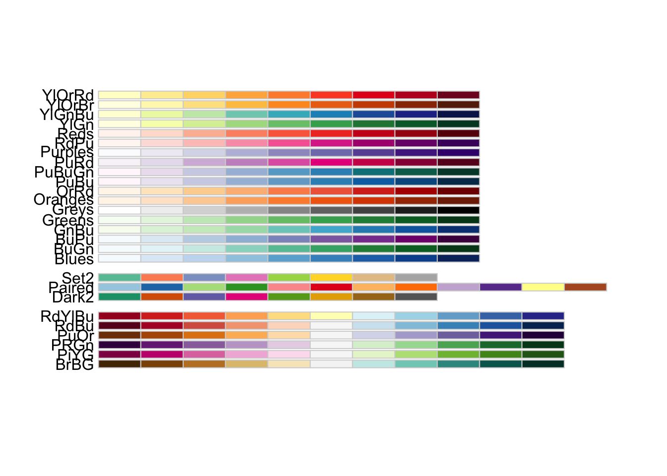

RColorBrewer’s colorblind friendly palettes.

PuBuGn <- brewer.pal(n = 9, name = "PuBuGn")
PuBuGn

[1] "#FFF7FB" "#ECE2F0" "#D0D1E6" "#A6BDDB" "#67A9CF" "#3690C0" "#02818A"
[8] "#016C59" "#014636"

barplot(rep(1, length(PuBuGn)), col = PuBuGn)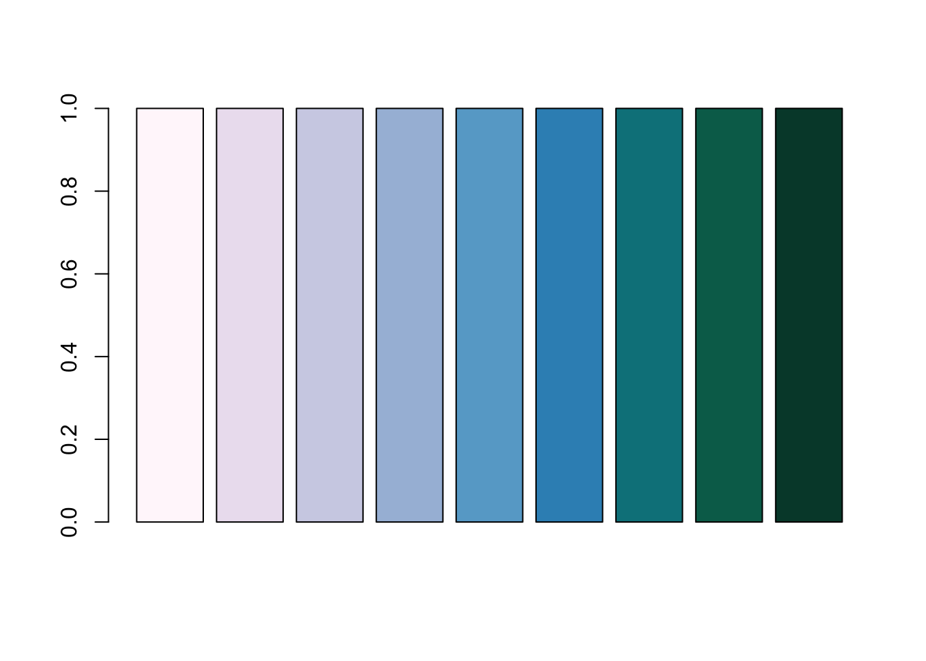

A barplot demonstating the RColorBrewer’s PuBuGn palette.

colorspace R package

The colorspace R package is a complex tool with a simple interface whose core functionality is to “carry out mapping between assorted color spaces including RGB, HSV, HLS, CIEXYZ, CIELUV, HCL (polar CIELUV), CIELAB and polar CIELAB” (directly from the package description). It also provides something handy: an emulator of color vision defficiencies both through the command line and colorspace’s GUIs. See the color vision deficiency emulation article from the colorspace web pages.

Accessing the colospace shiny GUI is as simple as

library("colorspace")
hcl_wizard()

On the GUI, you can choose to see how the colors look like to someone with normal, deutan (green-blindness), protan (red-blindness) and tritan (blue-blindness) vision, or even wholly desaturate the colours to see if you can distinguish them from each other. The functions deutan(), protan(), and tritan() take as input a vector of colors and return the hex color codes of how that colour looks like depending on the severity of each vision deficiency. For example,

severity <- seq(0, 1, 0.1)
protan_greens <- sapply(severity, protan, col = "green")
barplot(rep(1, length(severity)), col = protan_greens, xlab = "severity of protanopia")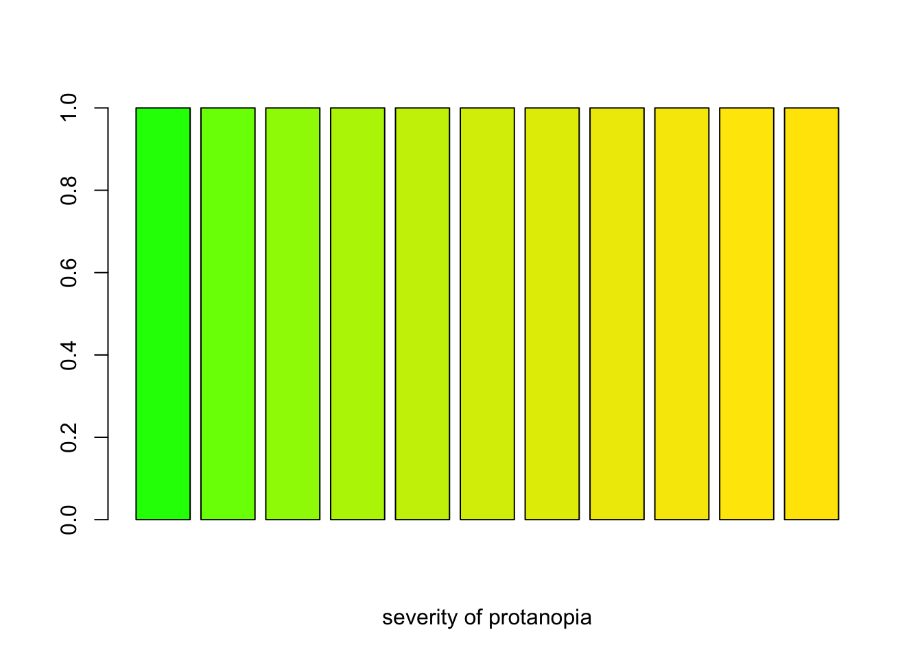

A barplot demosntrating how R’s color ‘green’ looks like for varying severity of protanopia.

viridis R package

The palettes provided by the viridis R package are designed to be “perfectly perceptually-uniform, both in regular form and also when converted to black-and-white. They are also designed to be perceived by readers with the most common form of color blindness (all color maps in this package) and color vision deficiency (‘cividis’ only)” (directly from the package description). For example, the often-encountered rainbow palette scores very low when displaying information to individuals with color deficiencies:

rain <- rainbow(n = 30)
par(mfrow = c(2, 2), mar = c(2, 2, 2, 2))
barplot(rep(1, length(rain)), col = rain, main = "no deficiency")
barplot(rep(1, length(rain)), col = protan(rain), main = "protanopia (red-blindness)")
barplot(rep(1, length(rain)), col = deutan(rain), main = "deutanopia (green-blindness)")
barplot(rep(1, length(rain)), col = tritan(rain), main = "tritanopia (blue-blindness)")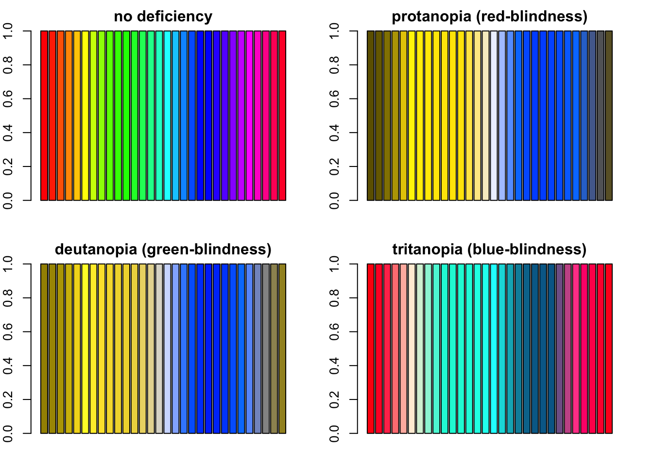

Four barplots demonstating how R’s rainbow palette looks like with severe protanopia, deutanopia and tritanopia.

On the other hand, viridis’ inferno works well (you should see a sequence of 30 bars from darker to lighter regardless of which of the four barplots you are looking at).

library("viridis")

Loading required package: viridisLite

inferno <- inferno(n = 30)
par(mfrow = c(2, 2), mar = c(2, 2, 2, 2))
barplot(rep(1, length(inferno)), col = inferno, main = "no deficiency")
barplot(rep(1, length(inferno)), col = protan(inferno), main = "protanopia (red-blindness)")
barplot(rep(1, length(inferno)), col = deutan(inferno), main = "deutanopia (green-blindness)")
barplot(rep(1, length(inferno)), col = tritan(inferno), main = "tritanopia (blue-blindness)")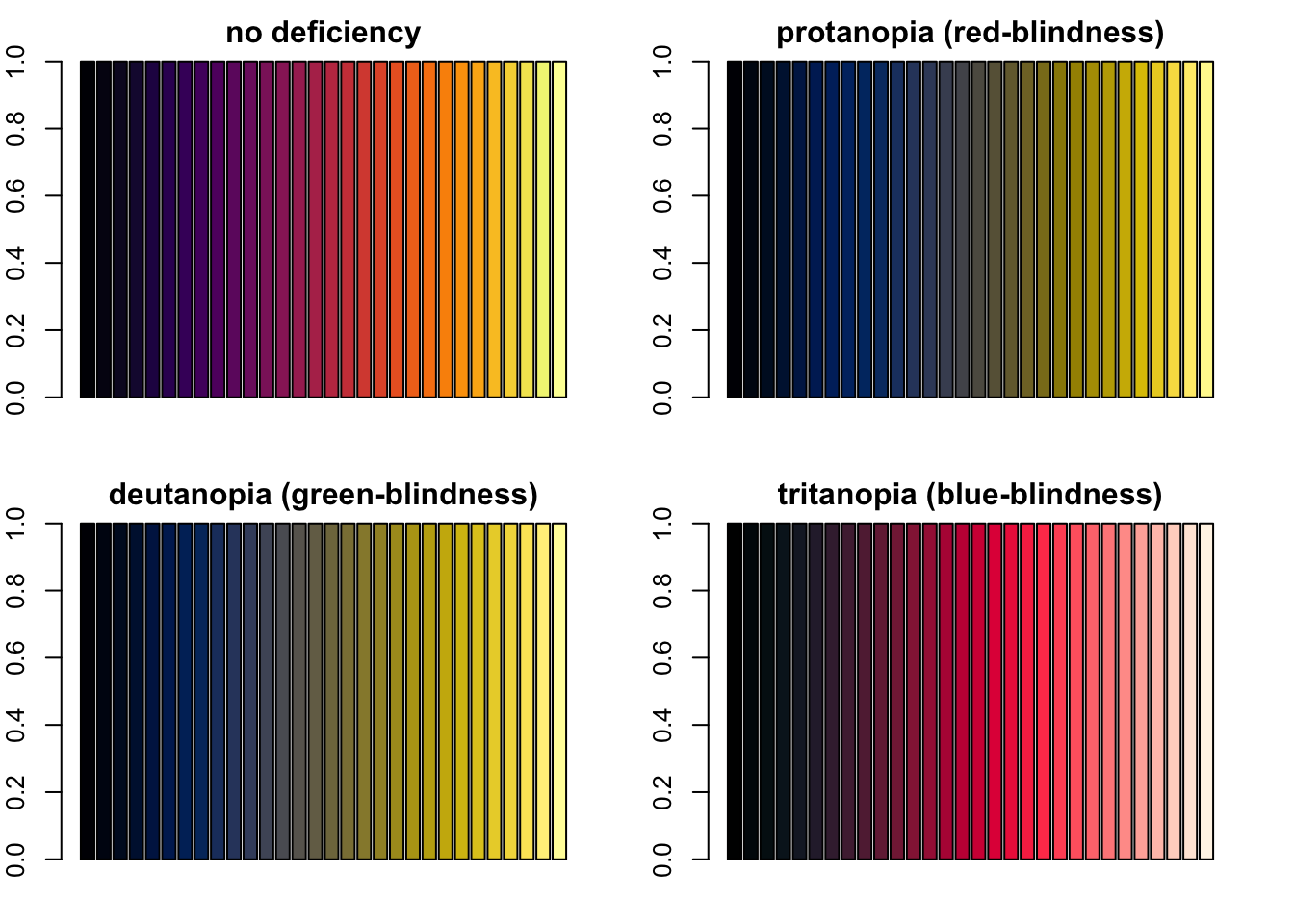

Four barplots demonstating how viridis’ inferno palette looks like with severe protanopia, deutanopia and tritanopia.