The R code reproducing the analyses and simulations presented on the slide deck is all embedded on the slides. Just click “[R Code]” wherever it appears.
From this point onward, when evaluating a code chunk, it is assumed that all previous chunks have been successfully evaluated.
R packages
The code on the slides rely on R version 4.5.3 (2026-03-11) and the packages
package
version
mclust
6.1.2
You can load them (and install them if you do not have them already) by doing
pkgs <-c("mclust")for (pkg in pkgs)if (!require(pkg, character.only =TRUE))install.packages(pkg)
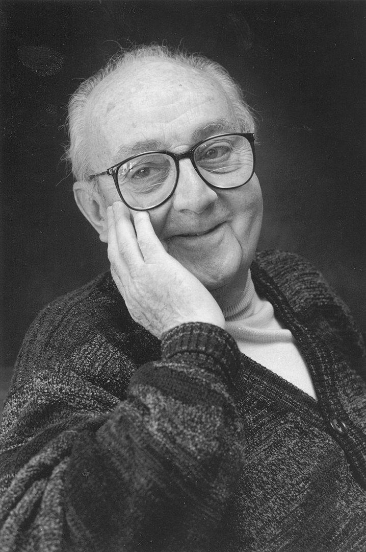
George Box (1919 – 2013)
Remember that all models are wrong; the practical question is how wrong do they have to be to not be useful.
in Box and Draper (1987). Empirical Model-Building and Response Surfaces, p. 74
Latent variable models
Latent variables: setting
Many statistical models simplify when written in terms of unobserved latent variable\(U\) in addition to the observed data \(Y\). The latent variable
may really exist: for example, when \(Y = I(U > c)\) for some continuous \(U\) (“do you earn less than c per year?”);
may be human construct: for example, something called IQ is said to underlie scores on intelligence tests, but is IQ just a cultural construct? (“Mismeasure of man” debate, etc.);
may just be a mathematical / computational device: for example, latent variables are used in the implementation of MCMC or EM algorithms.
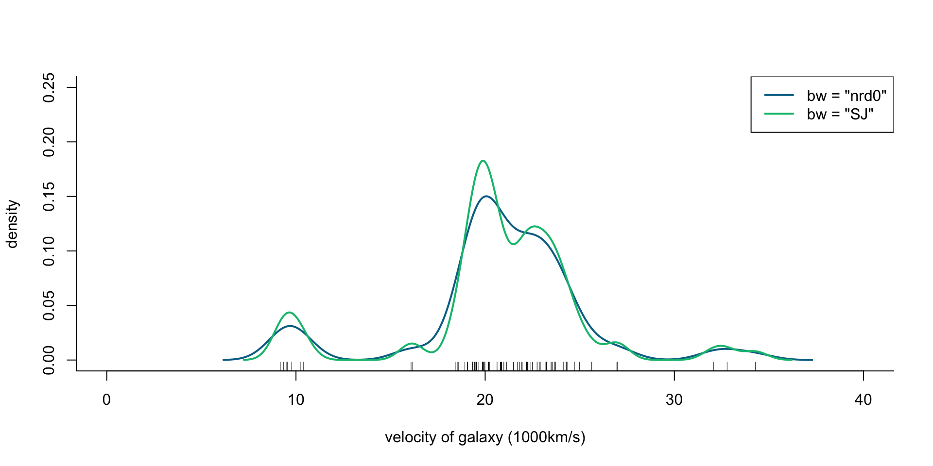
Velocity of galaxies: ?MASS::galaxies
The velocities, in km/sec, of 82 galaxies, moving away from our own galaxy, from 6 well-separated conic sections of an ‘unfilled’ survey of the Corona Borealis region. Multimodality in such surveys is evidence for voids and superclusters in the far universe.
If galaxies are indeed super-clustered the distribution of their velocities estimated from the red-shift in their light-spectra would be multimodal, and unimodal otherwise
data("galaxies", package ="MASS")## Fix typo see `?galaxies`galaxies[78] <-26960galaxies
## Rescale to 1000km/sgalaxies <- galaxies /1000plot(x =c(0, 40), y =c(0, 0.25), type ="n", bty ="l",xlab ="velocity of galaxy (1000km/s)", ylab ="density")rug(galaxies)lines(density(galaxies, bw ="nrd0"), col = cols[2], lwd =2)lines(density(galaxies, bw ="SJ"), col = cols[3], lwd =2)legend("topright", legend =c('bw = "nrd0"', 'bw = "SJ"'),col = cols[2:3], lty =1, lwd =2)
Figure 1: Density of galaxy velocities in 1000km/s, using two kernel density estimators with gaussian kernel but different bandwidth selection procedures.
Latent variable models
Let \([U], D\) denote discrete random variables, and \((U), X\) continuous ones.
\([U] \to X\) or \([U]\to D\)
\((U) \to D\)
\((U)\to X\) or \((U)\to D\)
finite mixture models
censoring
generalized nonlinear mixed models
hidden Markov models
truncation
exploratory / confirmatory factor analysis
changepoint models
item-response theory models
\(\vdots\)
\(\vdots\)
\(\vdots\)
Example: probit regression
A generalized linear model for binary data with a probit link function can be written as \[
\begin{aligned}
U_i & \stackrel{\text{ind}}{\sim}\mathop{\mathrm{N}}(x_i^\top \beta, 1) \\
Y_i & = I(U_i \geq 0)
\end{aligned}
\]
The log-likelihood of the probit regression model is then \[
\sum_{i = 1}^n \left\{ y_i \log \Phi(x_i^\top \beta) + (1 - y_i)\log\{1 - \Phi(x^\top\beta)\} \right\}
\]
Different assumptions for the distribution of the latent variable \(U\) give rise to different models (e.g. logistic distribution gives rise to logistic regression, extreme-value distribution to complementary log-log regression, etc.).
Finite mixture models
Setting
Observations are taken from a population composed of distinct sub-populations, but it is unknown from which of those sub-populations the observations come from (e.g. the galaxy velocities data).
\(p\)-component finite mixture model
The \(p\)-component finite mixture model has density or probability mass function \[
f(y \,;\,\pi, \theta) = \sum_{r=1}^p \pi_r f_r(y \,;\,\theta) \quad (0\leq \pi_r\leq 1 ; \sum_{r=1}^p \pi_r = 1)
\] where \(\pi_r\) is the probability that \(y\) is from the \(r\)th component, and \(f_r(y \,;\,\theta)\) is its density or probability mass function conditional on this event (component density).
Finite mixture models
Latent variable
\[
U = \left\{\begin{array}{ll}
1\,, & \text{with probability } \pi_1 \\
2\,, & \text{with probability } \pi_2 \\
\vdots \\
p\,, & \text{with probability } \pi_p \\
\end{array}\right.
\]
A widely used class of models for density estimation and clustering. It is often assumed that the number of components \(p\) is unknown.
Such models are non-regular for likelihood inference:
The ordering of components is non-identifiable. In other works, charging the order of the components does not change model.
Setting \(\pi_r = 0\) eliminates the unknown parameters in \(f_r(y \,;\,\pi, \theta)\)
Depending on the specification of the component distribution, the maximum of the log-likelihood can be \(+\infty\), and can be achieved for various \(\theta\).
Typically, implementations use constraints on the parameters to overcome such issues.
Expectation-Maximization
Aim
The Expectation-Maximization (EM) algorithm is a powerful tool that allows to use the observed value \(y\) of \(Y\) for inference on \(\theta\) when we cannot easily compute \[
f(y \,;\,\theta) = \int f(y\mid u \,;\,\theta) f(u \,;\,\theta) du
\]
It proceeds by exploiting the latent variables.
EM Derivation
Complete data log-likelihood
Suppose that we observe \(U\). Then, the Bayes theorem gives that the complete data log-likelihood is \[
\log f(y, u \,;\,\theta) = \log f(y \,;\,\theta) + \log f(u \mid y \,;\,\theta)
\tag{1}\]
Incomplete data log-likelihood
The incomplete data log-likelihood (also known as observable data log-likelihood) is simply \[
\ell(\theta) = \log f(y \,;\,\theta)
\]
EM Derivation: \(Q\) function
\(Q(\theta\,;\,\theta')\)
Take expectations in both sides of (1) with respect to \(f(u \mid y \,;\,\theta')\). We have \[
\underbrace{\mathop{\mathrm{E}}\left( \log f(Y, U \,;\,\theta) \mid Y = y \,;\,\theta'\right)}_{Q(\theta\,;\,\theta')} =
\ell(\theta) + \overbrace{\mathop{\mathrm{E}}\left( \log f(U \mid Y \,;\,\theta)\mid Y = y \,;\,\theta'\right)}^{C(\theta \,;\,\theta')}
\tag{2}\]
Behaviour of \(Q(\theta \,;\,\theta')\) as a function of \(\theta\)
\[
\begin{aligned}
C(\theta \,;\,\theta') - C(\theta' \,;\,\theta') & = \mathop{\mathrm{E}}\left( \log \frac{f(U \mid Y \,;\,\theta)}{f(U \mid Y \,;\,\theta')} \mid Y = y \,;\,\theta'\right) \\
& \le \log \mathop{\mathrm{E}}\left( \frac{f(U \mid Y \,;\,\theta)}{f(U \mid Y \,;\,\theta')} \mid Y = y \,;\,\theta'\right) \\
& = \log \int \frac{f(u \mid Y = y \,;\,\theta)}{f(u \mid Y =y \,;\,\theta')} f(u \mid Y = y \,;\,\theta') du \\
& = \log \int f(u \mid Y = y \,;\,\theta) du = 0 \\
& \implies C(\theta' \,;\,\theta')\geq C(\theta \,;\,\theta')
\end{aligned}
\]
Under mild smoothness conditions, \(C(\theta \,;\,\theta')\) has a stationary point at \(\theta := \theta'\).
So, if \(Q(\theta \,;\,\theta')\) is stationary at \(\theta := \theta'\), (2) implies that so too is \(\ell(\theta)\)!
EM algorithm for maximizing \(\ell(\theta)\)
Starting from an initial value \(\theta'\) of \(\theta\)
Expectation (E) step
Compute \(Q(\theta \,;\,\theta') = \mathop{\mathrm{E}}\left( \log f(Y,U \,;\,\theta)
\mid Y = y \,;\,\theta'\right)\).
Maximization (M) step
With \(\theta'\) fixed, maximize \(Q(\theta \,;\,\theta')\) with respect to \(\theta\), and let \(\theta^\dagger\) be the maximizer.
Check convergence, based on the size of \(\ell(\theta^\dagger) -
\ell(\theta')\) if available, or \(\|\theta^\dagger - \theta'\|\), or both.
If the algorithm has converged stop and return \(\theta^\dagger\) as the value of the maximum likelihood estimator \(\hat\theta\). Otherwise, set \(\theta' := \theta^\dagger\) and go to 1.
The M-step ensures that \(Q(\theta^\dagger \,;\,\theta') \geq Q(\theta'
\,;\,\theta')\), so (3) implies that \(\ell(\theta^\dagger) \geq \ell(\theta')\).
\[
\LARGE\Downarrow
\]
The log likelihood never decreases between EM iterations!
EM algorithm: notes on convergence
If \(\ell(\theta)\) has only one stationary point, and \(Q(\theta \,;\,
\theta')\) eventually reaches a stationary value at \(\hat\theta\), then \(\hat\theta\) must maximize \(\ell(\theta)\).
Otherwise, the algorithm may converge to a local maximum of the log likelihood or to a saddlepoint.
EM never decreases the log likelihood so it is, generally, more stable than gradient-descent-type algorithms. The rate of convergence depends on closeness of \(Q(\theta \,;\,\theta')\) and \(\ell(\theta)\).
Missing information principle
Observed information equals the complete-data information minus the missing information.
EM’s rate of convergence is slow if the missing information is a high proportion of the total, or if the largest eigenvalue of \(I_c(\theta
\,;\,y)^{-1}I_m(\theta \,;\,y) \approx 1\).
Example: negative binomial
If \[
\begin{aligned}
Y \mid U = u & \sim \mathop{\mathrm{Poisson}}(u) \\
U & \sim \mathop{\mathrm{Gamma}}(\nu, \theta / \nu)
\end{aligned}
\] (i.e. \(\mathop{\mathrm{E}}(U) = \theta\) and \(\mathop{\mathrm{var}}(U) = \theta^2 / \nu\))
Then1, \[
Y \sim \mathop{\mathrm{NegativeBinomial}}(\nu, \frac{\nu}{\theta + \nu})
\]
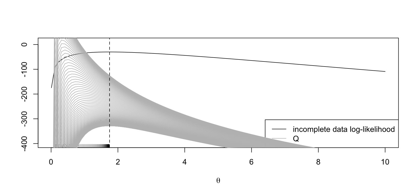
Suppose \(\nu = 20\) is known and we wish to estimate \(\theta\).
Example: negative binomial1
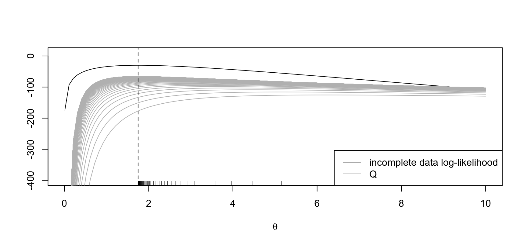
inc_loglik <-function(theta, nu, y) {sum(dnbinom(y, nu, nu / (theta + nu), log =TRUE))}Q <-function(theta, theta_d, nu, y) {sum(-(1+ nu / theta) * (y + nu) / (1+ nu / theta_d) - nu *log(theta))}theta_dagger <-function(theta_d, nu, y) { theta_d * (mean(y) + nu) / (theta_d + nu)}set.seed(123)nu <-20theta_true <-1.5y <-rnbinom(20, nu, nu / (theta_true + nu))theta_grid <-seq(0.01, 10, length =100)inc_ll <-sapply(theta_grid, inc_loglik, nu = nu, y = y)maxit <-400theta_start <- theta_d <-0.1## Scaling factor for nice plotsscl <-2plot(theta_grid, inc_ll, type ="l", ylim =c(-400, 10),ylab ="", xlab =expression(theta))legend("bottomright", legend =c("incomplete data log-likelihood", "Q"),col =c("black", "grey"), lty =1)for (r in1:maxit) { Q1 <-sapply(theta_grid, Q, theta_d = theta_d, nu = nu, y = y) / sclif (r %%4==0) {points(theta_grid, Q1, type ="l", col ="grey") theta_d <-theta_dagger(theta_d, nu, y)rug(theta_d) }}abline(v =mean(y), lty =2)
The maximum of the incoplete-data log-likelihood is at \(\hat\theta := 1.75\). EM starting at \(\theta' = 0.1\).
Example: negative binomial1
theta_start <- theta_d <-8## Scaling factor for nice plotsscl <-10plot(theta_grid, inc_ll, type ="l", ylim =c(-400, 10),ylab ="", xlab =expression(theta))legend("bottomright", legend =c("incomplete data log-likelihood", "Q"),col =c("black", "grey"), lty =1)for (r in1:300) { Q1 <-sapply(theta_grid, Q, theta_d = theta_d, nu = nu, y = y) / sclif (r %%4==0) {points(theta_grid, Q1, type ="l", col ="grey") theta_d <-theta_dagger(theta_d, nu, y)rug(theta_d) }}abline(v =mean(y), lty =2)
The maximum of the incoplete-data log-likelihood is at \(\hat\theta := 1.75\). EM starting at \(\theta' = 8\).
EM for mixture models
E-step for mixture models
The contribution to the complete data log-likelihood (assuming that we know from what component \(y\) is from) of a mixture model is \[
\log f(y, u \,;\,\pi, \theta) = \sum_{r=1}^p I(u=r)\left\{ \log \pi_r + \log f_r(y \,;\,\theta)\right\}
\]
We need the expectation of \(\log f(y,u \,;\,\theta)\) over distribution of \(U \mid Y = y\) at \(\pi'\) and \(\theta'\), that is \[
w_r(y \,;\,\pi', \theta') = P(U = r \mid Y = y \,;\,\pi', \theta') = {\pi'_r f_r(y \,;\,\theta')\over \sum_{s=1}^p \pi'_s f_s(y \,;\,\theta')} \quad (r=1,\ldots,p)
\tag{4}\] which is the weight attributable to component \(r\) given observation \(y\).
The only quantities depending on \(U\) in the completed data log-likelihood are \(I(U = r)\). So, \[
\begin{aligned}
\mathop{\mathrm{E}}(I(U = r) \mid Y = y \,;\,\pi', \theta') & = P(U = r \mid Y = y \,;\,\pi', \theta') = w_r(y \,;\,\pi', \theta')\\
\end{aligned}
\]
E-step for mixture models
The expected value of the complete-data log likelihood based on a random sample \((y_1, u_1), \ldots, (y_n, u_n)\) is \[
\begin{aligned}
Q(\pi, \theta \,;\,\pi', \theta') & = \sum_{j=1}^n \sum_{r=1}^p w_r(y_j \,;\,\pi', \theta')\left\{ \log\pi_r + \log
f_r(y_j \,;\,\theta)\right\}\\
&= \sum_{r=1}^p \left\{ \sum_{j=1}^n w_r(y_j \,;\,\pi', \theta')\right\}\log\pi_r +
\sum_{r=1}^p \sum_{j=1}^n w_r(y_j \,;\,\pi', \theta')\log f_r(y_j \,;\,\theta)
\end{aligned}
\]
\(\pi_r\) do not usually appear in the component density \(f_r\). So, \[
\left\{\pi_r^\dagger\right\} = \arg\max A(\pi) = \left\{\frac{1}{n} \sum_{j = 1}^n w_r(y_j \,;\,\pi', \theta')\right\}
\] which are the average weights given the data for each component.
M-step for mixture models
Iterates for \(\theta\)
\(f_r\) do not depend on \(\pi_r\). So, \[
\theta^\dagger = \arg\max B(\theta)
\]
Example: Univariate normal components1
If \(f_r\) is the normal density with mean \(\mu_r\) and variance \(\sigma^2_r\), simple calculations give that the M-step results in the weighted estimates \[
\mu_r^\dagger = {\sum_{j=1}^n w_r(y_j \,;\,\pi', \theta') y_j\over \sum_{j=1}^n
w_r(y_j \,;\,\pi', \theta')}\,, \quad
\sigma^{2\dagger}_r = {\sum_{j=1}^n w_r(y_j \,;\,\pi', \theta')(y_j-\mu_r^\dagger)^2\over \sum_{j=1}^n
w_r(y_j \,;\,\pi', \theta')} \quad (r=1,\ldots,p)
\]
Velocity of galaxies: Mixture of normal distributions
Let’s fit a mixture model with normal component densities, where each component has its own mean and variance. This can be done using the mclust R package, which provides the EM algorithm for (multivariate) gaussian mixture models.
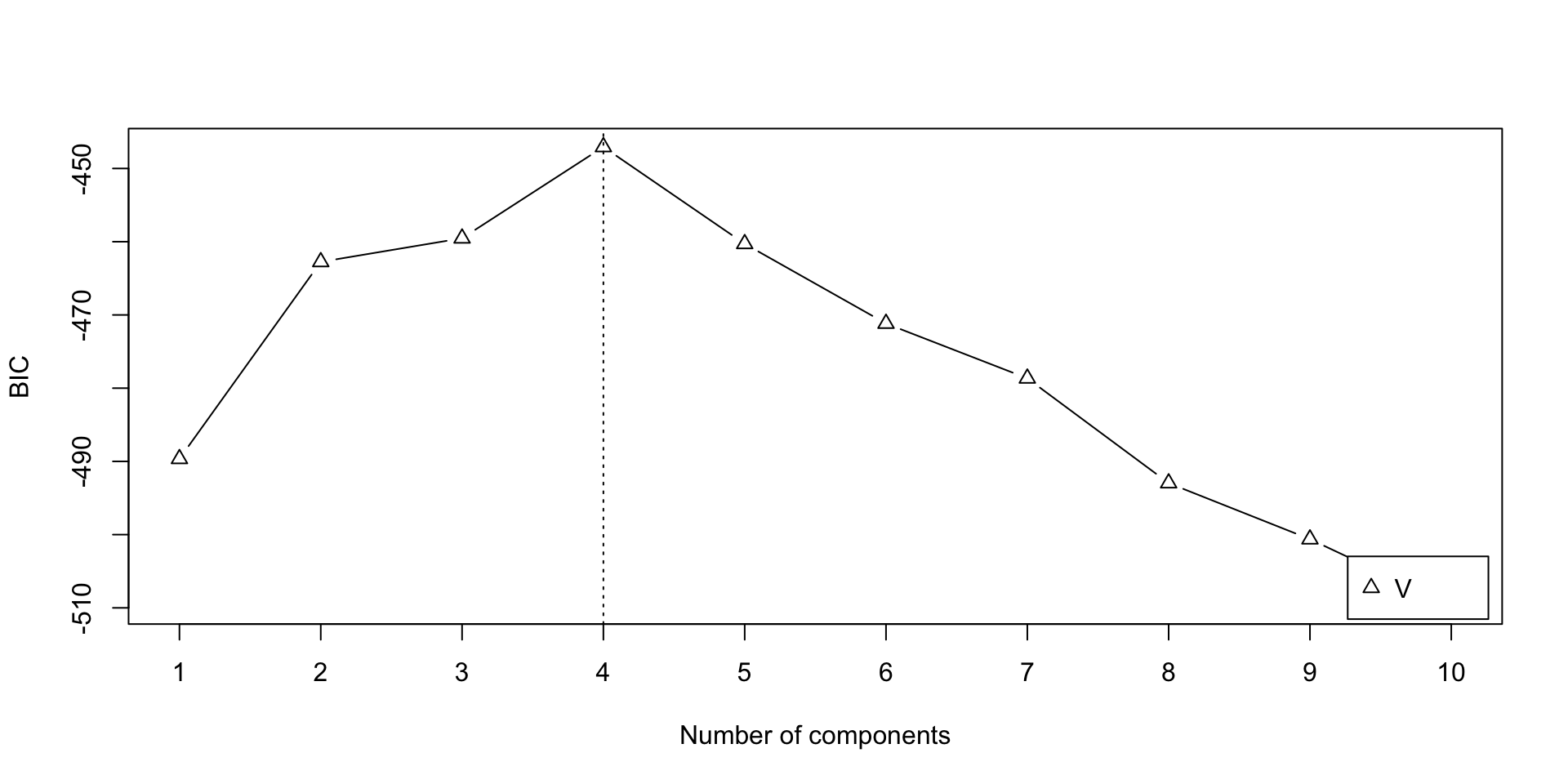
gal_mix <-Mclust(galaxies, G =1:10, modelNames ="V")plot(gal_mix, what ="BIC")abline(v =4, lty =3)
[mclust reports the negative of the BIC as we defined it]
Velocity of galaxies: Density estimation
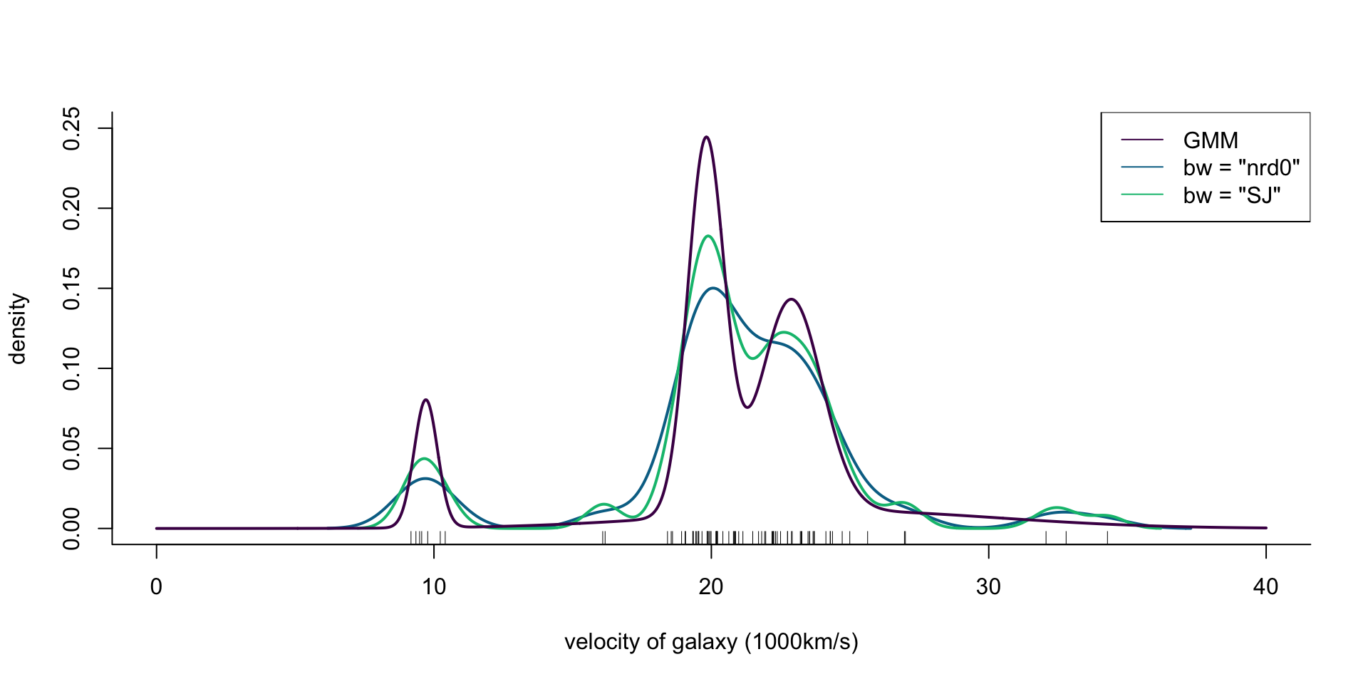
plot(x =c(0, 40), y =c(0, 0.25), type ="n", bty ="l",xlab ="velocity of galaxy (1000km/s)", ylab ="density")rug(galaxies)lines(density(galaxies, bw ="nrd0"), col = cols[2], lwd =2)lines(density(galaxies, bw ="SJ"), col = cols[3], lwd =2)legend("topright", legend =c('bw = "nrd0"', 'bw = "SJ"'),col = cols[2:3], lty =1, lwd =2)
Figure 2: Density of galaxy velocities in 1000km/s, using two kernel density estimators with gaussian kernel but different bandwidth selection procedures, and a mixture of 4 normal densities.
Figure 3: Density of galaxy velocities in 1000km/s, using two kernel density estimators with gaussian kernel but different bandwidth selection procedures, and a mixture of 4 normal densities.
Clustering and assignment uncertainty
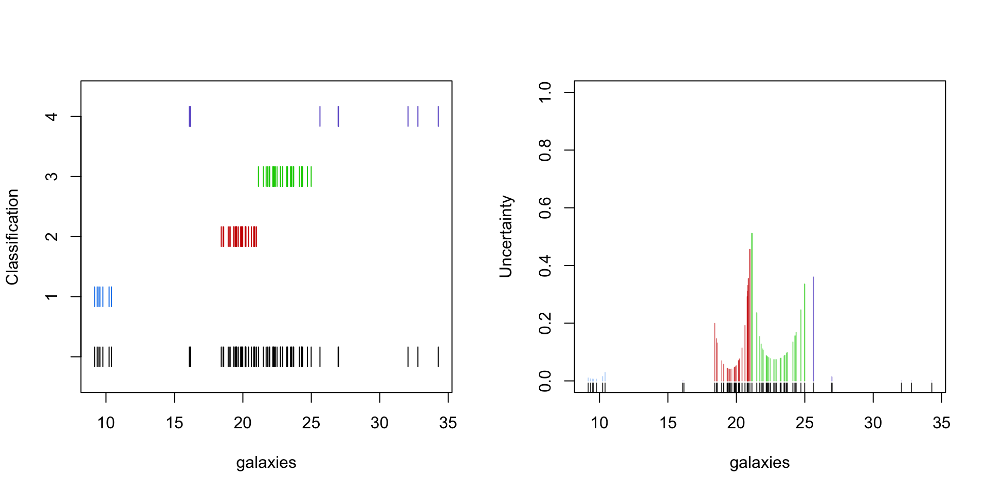
Apart from computation convenient, EM for mixture models results in some useful byproducts.
The weights (4) from the E-step can be used to determine - the component at which the observation is assigned to - the uncertainty about that assignment
par(mfrow =c(1, 2))plot(gal_mix, what ="classification")plot(gal_mix, what ="uncertainty")
Exponential families
Suppose that the complete-data log likelihood has the form \[
\log f(y,u \,;\,\theta) = s(y,u)^\top\theta - \kappa(\theta) + c(y, u)
\]
Ignoring \(c(y, u)\), the M-step of the EM algorithm involves maximizing \[
Q(\theta \,;\,\theta') = \left\{\mathop{\mathrm{E}}\left( s(y,U)\mid Y = y \,;\,\theta'\right)\right\}^\top \theta -
\kappa(\theta)
\] or, equivalently, solving for \(\theta\) the equation \[
\mathop{\mathrm{E}}\left( s(y,U)\mid Y=y \,;\,\theta'\right) = {\partial\kappa(\theta)\over\partial\theta}
\]
The likelihood equation for \(\theta\) based on the complete data is \(s(y,u) = \partial\kappa(\theta)/\partial\theta\).
\[\Large\Downarrow\]
EM simply replaces \(s(y , u)\) by its conditional expectation \(\mathop{\mathrm{E}}\left(
s(y,U) \mid Y = y \,;\,\theta'\right)\) and solves the likelihood equation. A routine to fit the complete-data model can readily be adapted for missing data if the conditional expectations are available.
Bilmes, J. A. (1998). A gentle tutorial of the EM algorithm and its application to parameter estimation for gaussian mixture and hidden markov models. 15.
McLachlan, G. J., & Krishnan, T. (2008). The EM algorithm and extensions (2nd ed.). Wiley-Interscience.
Scrucca, L., Fop, M., Murphy, T., Brendan, & Raftery, A., E. (2016). Mclust 5: Clustering, classification and density estimation using gaussian finite mixture models. The R Journal, 8(1), 289. https://doi.org/10.32614/RJ-2016-021