The R code reproducing the analyses and simulations presented on the slide deck is all embedded on the slides. Just click “[R Code]” wherever it appears.
Parameters and covariates are allowed to have a nonlinear relationship.
The linear model results for \(\eta(x_i, \beta) = x_i^\top \beta\).
Nonlinear models
Parameter types in nonlinear models
Physical parameters that have particular meaning in the subject-area where the model comes from. Estimating the value of physical parameters, then, contributes to scientific understanding.
Tuning parameters that do not necessarily have any physical meaning. Their presence is justified as a simplification of a more complex underlying system. The aim when estimating them is to make the model represent reality as well as possible.
Specification of the nonlinear predictor
Mechanistically: prior scientific knowledge is incorporated into building a mathematical model for the mean response. That model can often be complex and \(\eta(x, \beta)\) may not be available in closed form.
Phenomenologically (empirically): a function \(\eta(x, \beta)\) may be posited that appears to capture the non-linear nature of the mean response.
Calcium uptake: ?SMPracticals::calcium
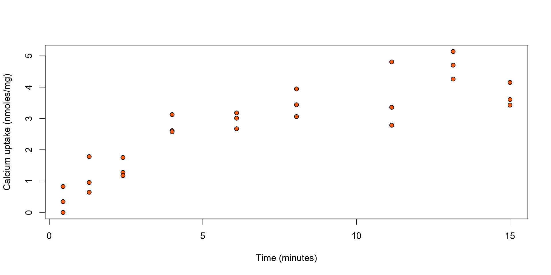
The uptake of calcium (in nmoles per mg) at set times (in minutes) by \(27\) cells in “hot” suspension.
data("calcium", package ="SMPracticals")plot(cal ~ time, data = calcium,xlab ="Time (minutes)",ylab ="Calcium uptake (nmoles/mg)",bg ="#ff7518", pch =21)
Figure 1: Calcium uptake against time.
Calcium uptake
A phenomenological model for growth curves
Assume that the rate of growth is proportional to the calcium remaining, i.e. \[
\frac{d \eta}{d t} = (\beta_0 - \eta) / \beta_1
\tag{1}\]
Solving the differential equation (1) with initial condition \(\eta(0,\beta) = 0\), gives \[
\eta(t, \beta) = \beta_0 \left( 1 - \exp \left( - t / \beta_1 \right) \right)
\]
Parameter interpretation
\(\beta_0\) is the calcium uptake after infinite time.
\(\beta_1\) controls the growth rate of calcium uptake.
Calcium uptake
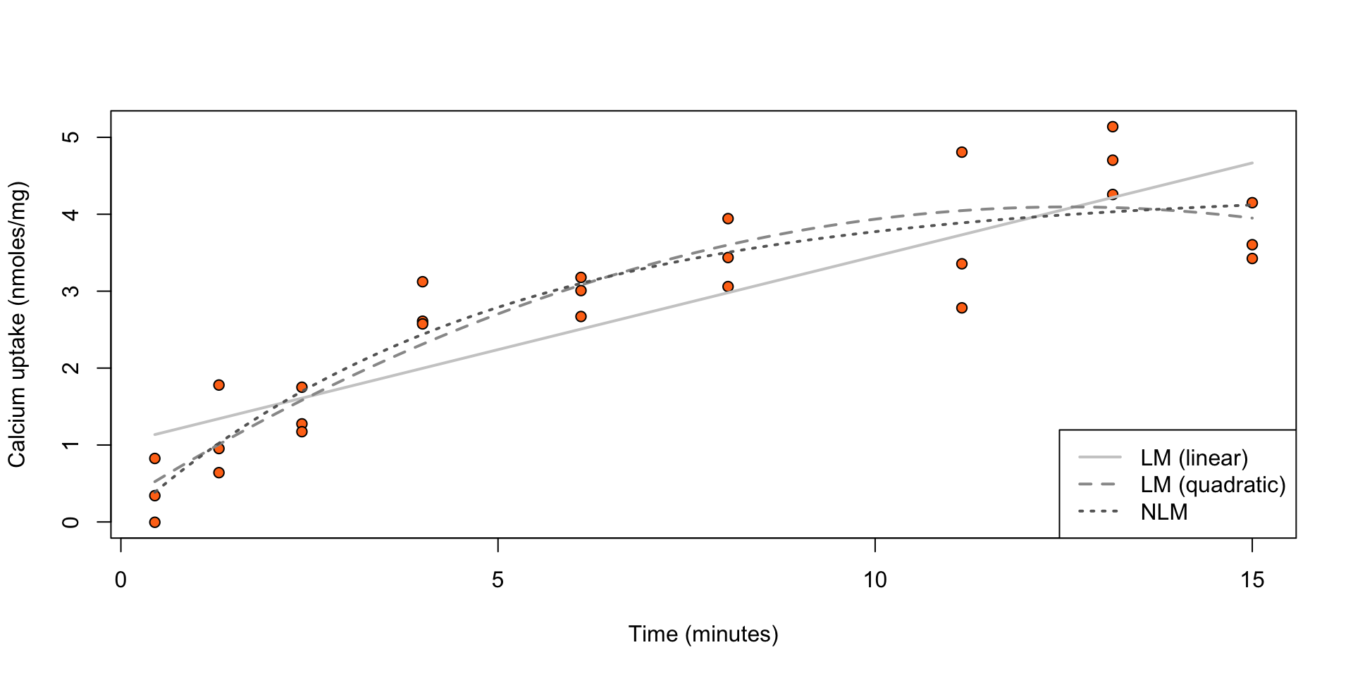
calc_lm1 <-lm(cal ~ time, data = calcium)calc_lm2 <-lm(cal ~ time +I(time^2), data = calcium)calc_nlm <-nls(cal~ beta0 * ( 1-exp(-time/beta1)), data = calcium,start =list(beta0 =5, beta1 =5))newdata <-data.frame(time =seq(min(calcium$time), max(calcium$time), length.out =100))pred_lm1 <-predict(calc_lm1, newdata = newdata)pred_lm2 <-predict(calc_lm2, newdata = newdata)pred_nlm <-predict(calc_nlm, newdata = newdata)plot(cal ~ time, data = calcium,xlab ="Time (minutes)",ylab ="Calcium uptake (nmoles/mg)",bg ="#ff7518", pch =21)lines(newdata$time, pred_lm1, col =gray(0.8), lty =1, lwd =2)lines(newdata$time, pred_lm2, col =gray(0.6), lty =2, lwd =2)lines(newdata$time, pred_nlm, col =gray(0.4), lty =3, lwd =2)legend("bottomright", legend =c("LM (linear)", "LM (quadratic)", "NLM"),col =gray(c(0.8, 0.6, 0.4)), lty =1:3, lwd =2)
Figure 2: Calcium uptake against time, overlaid by estimated expected uptake from three models with \(\eta(t, \beta) = \beta_1 + \beta_2 t\) (LM (linear)), \(\eta(t, \beta) = \beta_1 + \beta_2 x + \beta_3 t^2\) (LM (quadratic)), \(\eta(t, \beta) = \beta_0 ( 1 - \exp ( - t / \beta_1 ))\) (NLM).
Calcium uptake
A comparison of the three models in terms of number of parameters, maximized log-likelihood value, and AIC and BIC returns
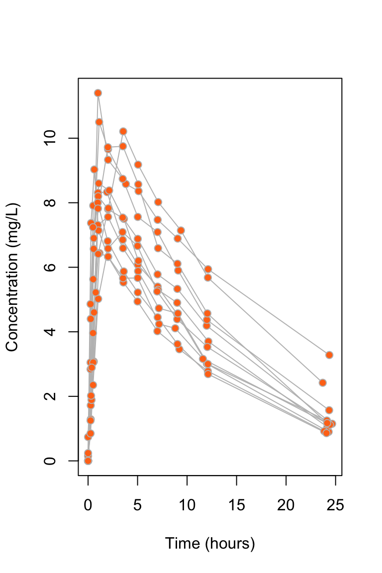
data("Theoph", package ="datasets")plot(conc ~ Time, data = Theoph, type ="n",ylab ="Concentration (mg/L)", xlab ="Time (hours)")for (i in1:30) { dat_i <-subset(Theoph, Subject == i)lines(conc ~ Time, data = dat_i, col ="grey")}points(conc ~ Time, data = Theoph, bg ="#ff7518", pch =21, col ="grey")
Figure 3: Concentration of theophylline against time for each of the individuals in the study.
Theophylline is an anti-asthmatic drug. An experiment was performed on \(12\) individuals to investigate the way in which the drug leaves the body. The study of drug concentrations inside organisms is called pharmacokinetics.
An oral dose was given to each individual at time \(t = 0\), and the concentration of theophylline in the blood was then measured at 11 time points in the next 25 hours.
Theophylline data: Compartmental models
Compartmental models are a common class of model used in pharmacokinetics studies.
If the initial dosage is \(D\), then pharmacokinetic model with a first-order compartment function is \[
\eta(\beta, D,t) = \frac{D \beta_1 \beta_2}{\beta_3(\beta_2 - \beta_1)} \left( \exp \left( - \beta_1 t\right) - \exp \left( - \beta_2 t\right)\right)\
\tag{2}\] where
\(\beta_1 > 0\): the elimination rate which controls the rate at which the drug leaves the organism.
\(\beta_2 > 0\): the absorption rate which controls the rate at which the drug enters the blood.
\(\beta_3 > 0\): the clearance which controls the volume of blood for which a drug is completely removed per time unit.
Theophylline data: Compartmental models
Since all the parameters are positive, and their estimation will most probably require a gradient descent step (e.g. what some of the methods in optim do), it is best to rewrite (2) in terms of \(\gamma_i = log(\beta_i)\). We can write \[
\eta'(\gamma, D, t) = \eta(\beta, D, t) = D \frac{\exp(-\exp(\gamma_1) t) - \exp(-\exp(\gamma_2) t)}{\exp(\gamma_3 - \gamma_1) - \exp(\gamma_3 - \gamma_2)}
\] where
\(\gamma_1 \in \Re\): the logarithm of the elimination rate.
\(\gamma_2 \in \Re\): the logarithm of the absorption rate.
\(\gamma_3 \in \Re\): the logarithm of the clearance.
Theophylline data: Fitting a pharmacokinetic model
We fit the model with predictor \(\eta'(\gamma, D_i,t_{ij})\) using nonlinear least-squares (nls() in R).
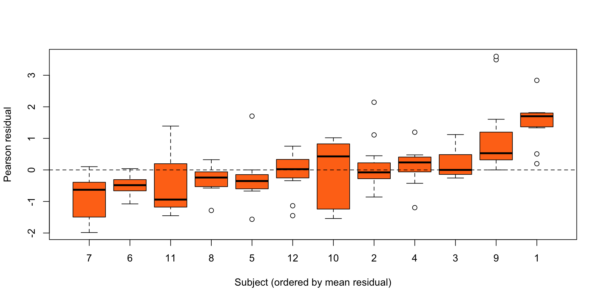
res <-residuals(pkm, type ="pearson")ord <-order(ave(res, Theoph$Subject))subj <- Theoph$Subject[ord]subj <-factor(subj, levels =unique(subj), ordered =TRUE)plot(res[ord] ~ subj,xlab ="Subject (ordered by mean residual)",ylab ="Pearson residual",col ="#ff7518", pch =21)abline(h =0, lty =2)
Figure 4: Residuals for each individual in the theopylline study from the nonlinear model \(Y_{ij} = \eta'(\gamma, D_i,t_{ij}) + \epsilon_{ij}\), \(\epsilon_{ij} \stackrel{\text{ind}}{\sim}{\mathop{\mathrm{N}}}(0,\sigma^2)\).
Clear evidence of unexplained differences between individuals.
Theophylline data: Fit assessment
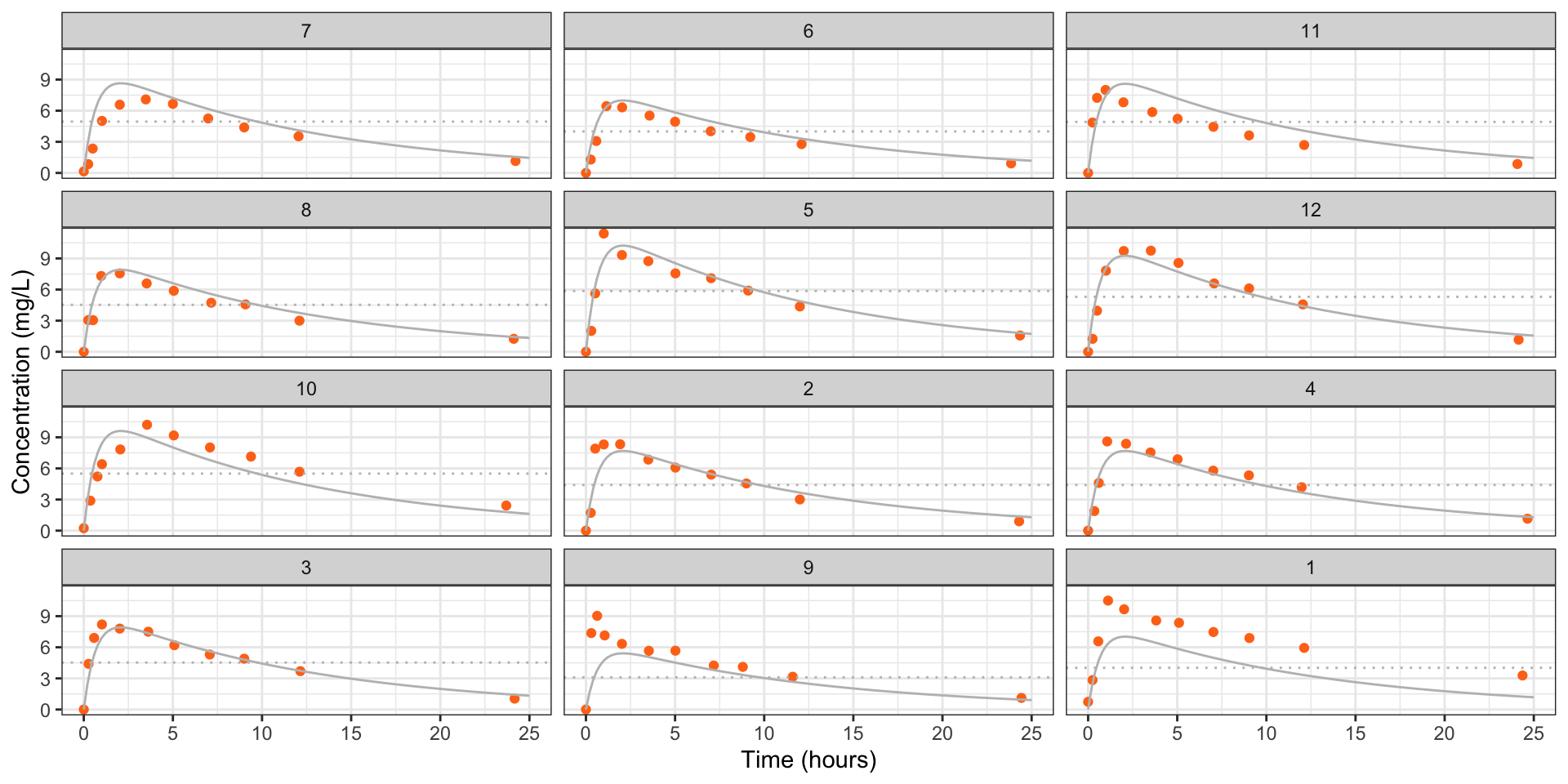
library("ggplot2")st <-unique(Theoph[c("Subject", "Dose")])pred_df <-as.list(rep(NA, nrow(st)))for (i inseq.int(nrow(st))) { pred_df[[i]] <-data.frame(Time =seq(0, 25, by =0.2),Dose = st$Dose[i],Subject = st$Subject[i])}pred_df <-do.call("rbind", pred_df)pred_df$conc <-predict(pkm, newdata = pred_df)## Order according to mean residualtheoph <-within(Theoph, Subject <-factor(Subject, levels =unique(subj), ordered =TRUE))fig_theoph <-ggplot(theoph) +geom_point(aes(Time, conc), col ="#ff7518") +geom_hline(aes(yintercept = Dose), col ="grey", lty =3) +facet_wrap(~ Subject, ncol =3) +labs(y ="Concentration (mg/L)", x ="Time (hours)") +theme_bw()fig_theoph +geom_line(data = pred_df, aes(Time, conc), col ="grey")
Figure 5: Estimated concentrations (grey) for each individual in the theopylline study from the nonlinear model \(Y_{ij} = \eta'(\gamma, D_i,t_{ij}) + \epsilon_{ij}\), \(\epsilon_{ij} \stackrel{\text{ind}}{\sim}{\mathop{\mathrm{N}}}(0,\sigma^2)\). The dotted line is the administered dose.
Accounting for heterogeneity between individuals seems worthwhile.
Nonlinear mixed effects models
\[
Y_{ij} = \eta(\beta + A b_i, x_{ij}) + \epsilon_{ij} \,, \quad \epsilon_{ij} \stackrel{\text{ind}}{\sim}{\mathop{\mathrm{N}}}(0,\sigma^2)\,, \quad b_i \stackrel{\text{ind}}{\sim}{\mathop{\mathrm{N}}}(0,\Sigma_b)
\] where \(\Sigma_b\) is a \(q \times q\) covariance matrix and \(A\) is a \(p
\times q\) matrix of zeros and ones, which determines which parameters are fixed and which are varying.
The linear mixed model is a special case of the nonlinear mixed model with \[
\eta(\beta + A b_i, x_{ij}) = x_{ij}^\top \left( \beta + A b_i\right)
= x_{ij}^\top \beta + x_{ij}^\top A b_i = x_{ij}^\top \beta + z_{ij}^\top b_i \,.
\]
A random intercept model results, if the first element of \(x_{ij}\) is \(1\) for all \(i\) and \(j\), \(q = 1\) and \(A = (1, 0, \ldots, 0)^\top\).
Theophylline data
We fit a nonlinear mixed model that allows all the parameters to vary across individuals, i.e. \(A = I_3\) using nmle() from the nlme R package.
Nonlinear mixed-effects model fit by maximum likelihood Model: fm Data: Theoph Log-likelihood: -173.3197 Fixed: gamma1 + gamma2 + gamma3 ~ 1 gamma1 gamma2 gamma3 0.4514709 -2.4326961 -3.2144616 Random effects: Formula: list(gamma1 ~ 1, gamma2 ~ 1, gamma3 ~ 1) Level: Subject Structure: General positive-definite, Log-Cholesky parametrization StdDev Corr gamma1 0.6376525 gamma1 gamma2gamma2 0.1310314 0.012 gamma3 0.2511740 -0.089 0.995Residual 0.6818382 Number of Observations: 132Number of Groups: 12
Theophylline data
Let’s consider the model with random effects with means \(\gamma_1\) and \(\gamma_3\), and just a population parameter for the logarithm of the absorption rate.
\[
Y_{ij} = \eta'\left(
\begin{bmatrix}
\gamma_1 + b_{i1} \\ \gamma_2 \\ \gamma_3 + b_{i3}
\end{bmatrix},
D_i, t_{ij}\right) + \epsilon_{ij} \, \quad \epsilon_{ij} \stackrel{\text{ind}}{\sim}{\mathop{\mathrm{N}}}(0,\sigma^2)\,, \quad (b_{i1}, b_{i3})^\top \stackrel{\text{ind}}{\sim}{\mathop{\mathrm{N}}}(0,\Sigma_b)
\] This corresponds to the general form pf the nonlinear mixed effects model with \[
A = \begin{bmatrix}
1 & 0 \\
0 & 0 \\
0 & 1
\end{bmatrix} \quad \text{and} \quad
b_i = \begin{bmatrix}
b_{i1} \\ b_{i3}
\end{bmatrix}
\]
A comparison to the model with all effects varying across individuals gives
pkmR_2 <-update(pkmR, random = gamma1 + gamma3 ~1)anova(pkmR, pkmR_2)
       Model df      AIC      BIC    logLik   Test  L.Ratio p-value
pkmR       1 10 366.6395 395.4675 -173.3197
pkmR_2     2  7 368.0464 388.2260 -177.0232 1 vs 2 7.406881    0.06
Theophylline data
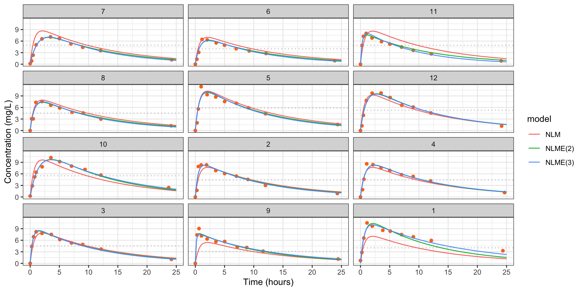
conc_nlm <- pred_df$concconc_nlme_2 <-predict(pkmR_2, newdata = pred_df)conc_nlme_3 <-predict(pkmR, newdata = pred_df)pred_df_all <- pred_df[c("Subject", "Dose", "Time")]pred_df_all <-rbind(data.frame(pred_df_all, conc = conc_nlm, model ="NLM"),data.frame(pred_df_all, conc = conc_nlme_2, model ="NLME(2)"),data.frame(pred_df_all, conc = conc_nlme_3, model ="NLME(3)"))fig_theoph +geom_line(data = pred_df_all, aes(Time, conc, color = model))
Figure 6: Estimated concentrations for each individual in the theopylline study from model (NLM), model with two effects varying (NLME(2)) and the model with all effects varying (NLM(3)). The dotted line is the administered dose.
Generalized nonlinear mixed effects models
Generalized nonlinear mixed effects models
The generalized nonlinear mixed effects model (GNLMM) assumes \[
Y_i \mid x_i, b_i \stackrel{\text{ind}}{\sim}\mathop{\mathrm{EF}}(\mu_i,\sigma^2)\,, \quad
\begin{bmatrix} g(\mu_1)\\\vdots \\ g(\mu_n) \end{bmatrix} =
\eta(\beta + A b_i, x_i) \,, \quad
b_i \stackrel{\text{ind}}{\sim}{\mathop{\mathrm{N}}}(0,\Sigma_b)
\] where \(\mathop{\mathrm{EF}}(\mu_i,\sigma^2)\) is an exponential family with mean \(\mu_i\) and variance \(\sigma^2 V(\mu_i) / m_i\).
Special cases
Linear model, nonlinear model, linear mixed effects model, nonlinear mixed effects model, generalized linear model, and generalized nonlinear model.
Fitting GNLMMs
As in GLMMs, the likelihood function may not have a closed form and needs approximation.
General-purpose optimizers may not converge to a global maximum of the likelihood.
Evaluating \(\eta(\beta, x)\) can be computationally expensive in some applications, like, for example, when \(\eta(\beta, x)\) is defined via a differential equation, which can only be solved numerically.
Bates, D. M., & Watts, D. G. (1988). Nonlinear regression analysis and its applications. Wiley.
Baty, F., Ritz, C., Charles, S., Brutsche, M., Flandrois, J.-P., & Delignette-Muller, M.-L. (2015). A toolbox for nonlinear regression in R: The package nlstools. Journal of Statistical Software, 66(5). https://doi.org/10.18637/jss.v066.i05
Lindstrom, M. J., & Bates, D. M. (1990). Nonlinear mixed effects models for repeated measures data. Biometrics, 46(3), 673–687. https://doi.org/10.2307/2532087
Pinheiro, J. C., & Bates, D. M. (1996). Unconstrained parametrizations for variance-covariance matrices. Statistics and Computing, 6(3), 289–296. https://doi.org/10.1007/BF00140873