APTS Statistical Modelling
Model Selection
14 April 2026
Space, time and feedback

Rooms
| Room | Building | |
|---|---|---|
| Lectures, Labs | A09, C13 | ESLC Building (54) |
| Breakouts rooms | C01 | ESLC Building (54) |
| Lunch, Tea and coffee | Foyer area | ESLC Building (54) |
Feedback
Close to or after the end of the week, please make sure you provide your feedback at
Code-chunks
The R code reproducing the analyses and simulations presented on the slide deck is all embedded on the slides. Just click “[R Code]” wherever it appears.
For example,
From this point onward, when evaluating a code chunk, it is assumed that all previous chunks have been successfully evaluated.
Velocity of galaxies: ?MASS::galaxies
R code
## Rescale to 1000km/s
galaxies <- galaxies / 1000
plot(x = c(0, 40), y = c(0, 0.25), type = "n", bty = "l",
     xlab = "velocity of galaxy (1000km/s)", ylab = "density")
rug(galaxies)
lines(density(galaxies, bw = "nrd0"), col = cols[2], lwd = 2)
lines(density(galaxies, bw = "SJ"), col = cols[3], lwd = 2)
legend("topright", legend = c('bw = "nrd0"', 'bw = "SJ"'),
       col = cols[2:3], lty = 1, lwd = 2)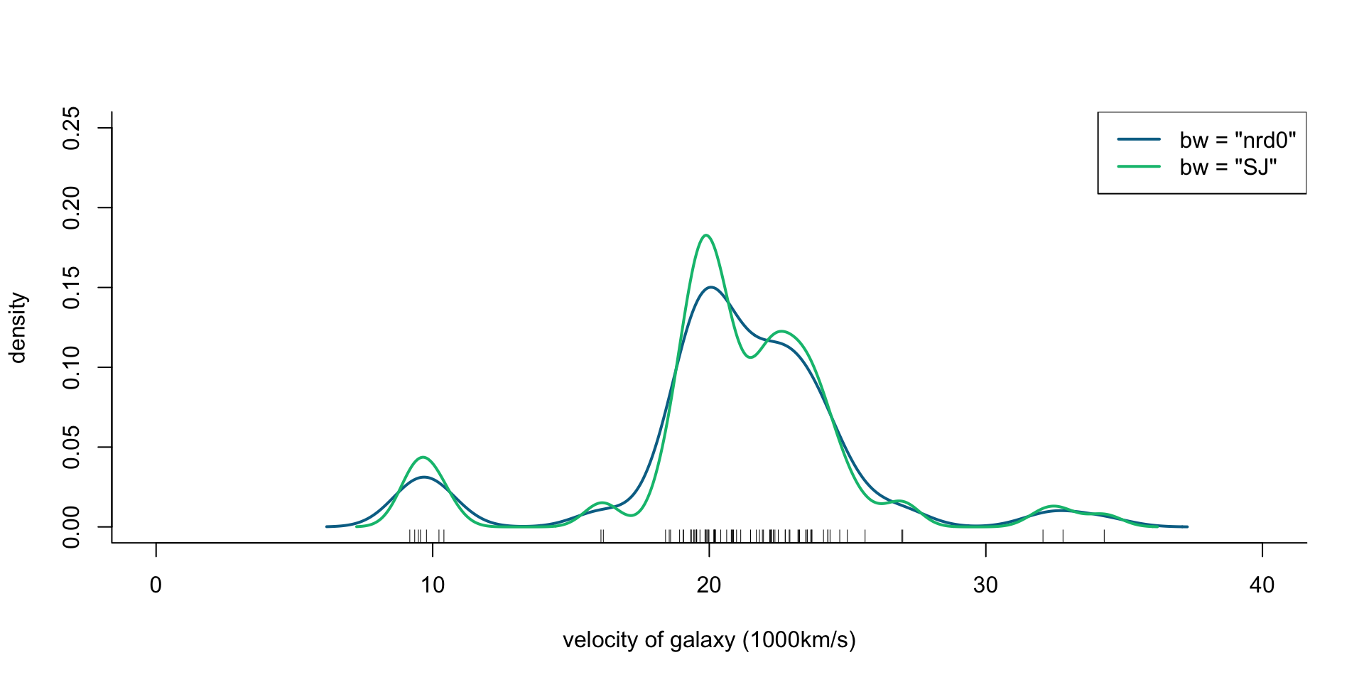
Figure 1: Density of galaxy velocities in 1000km/s, using two kernel density estimators with gaussian kernel but different bandwidth selection procedures.
Velocity of galaxies: Model selection for density estimation
R code
plot(x = c(0, 40), y = c(0, 0.25), type = "n", bty = "l",
     xlab = "velocity of galaxy (1000km/s)", ylab = "density")
rug(galaxies)
lines(density(galaxies, bw = "nrd0"), col = cols[2], lwd = 2)
lines(density(galaxies, bw = "SJ"), col = cols[3], lwd = 2)
legend("topright", legend = c('GMM - 1 component', 'bw = "nrd0"', 'bw = "SJ"'),
       col = cols, lty = 1)
ra <- seq(0, 40, length.out = 1000)
gal_mix <- Mclust(galaxies, G = 1, modelNames = "V")
lines(ra, dens(ra, modelName = "V", parameters = gal_mix$parameters),
      col = cols[1], lwd = 2)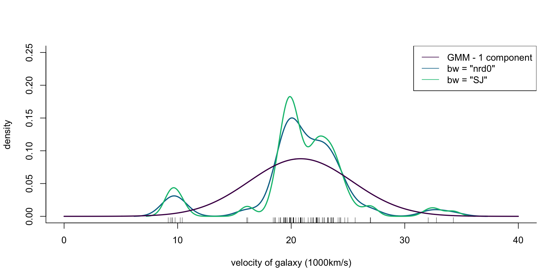
Figure 2: Density of galaxy velocities in 1000km/s, using two kernel density estimators with gaussian kernel but different bandwidth selection procedures, and 1 normal density.
Velocity of galaxies: Model selection for density estimation
R code
plot(x = c(0, 40), y = c(0, 0.25), type = "n", bty = "l",
     xlab = "velocity of galaxy (1000km/s)", ylab = "density")
rug(galaxies)
lines(density(galaxies, bw = "nrd0"), col = cols[2], lwd = 2)
lines(density(galaxies, bw = "SJ"), col = cols[3], lwd = 2)
legend("topright", legend = c('GMM - 2 components', 'bw = "nrd0"', 'bw = "SJ"'),
       col = cols, lty = 1)
ra <- seq(0, 40, length.out = 1000)
gal_mix <- Mclust(galaxies, G = 2, modelNames = "V")
lines(ra, dens(ra, modelName = "V", parameters = gal_mix$parameters),
      col = cols[1], lwd = 2)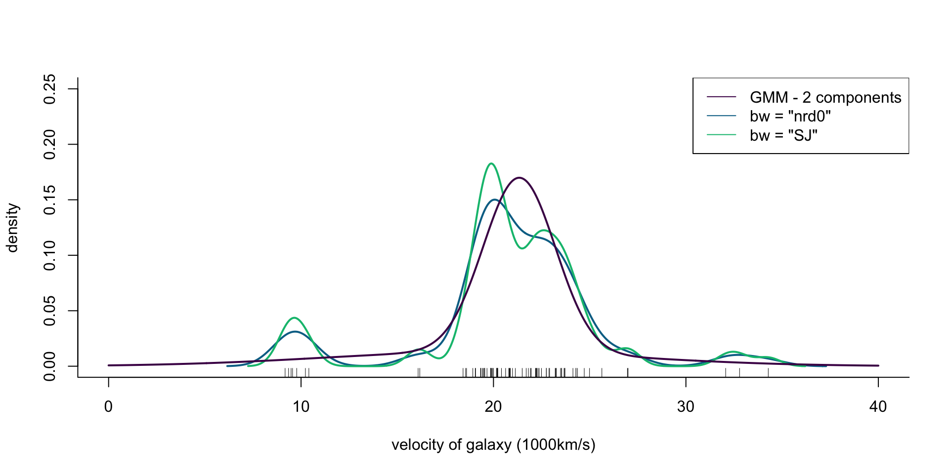
Figure 3: Density of galaxy velocities in 1000km/s, using two kernel density estimators with gaussian kernel but different bandwidth selection procedures, and a mixture of 2 normal densities.
Velocity of galaxies: Model selection for density estimation
R code
plot(x = c(0, 40), y = c(0, 0.25), type = "n", bty = "l",
     xlab = "velocity of galaxy (1000km/s)", ylab = "density")
rug(galaxies)
lines(density(galaxies, bw = "nrd0"), col = cols[2], lwd = 2)
lines(density(galaxies, bw = "SJ"), col = cols[3], lwd = 2)
legend("topright", legend = c('GMM - 3 components', 'bw = "nrd0"', 'bw = "SJ"'),
       col = cols, lty = 1)
ra <- seq(0, 40, length.out = 1000)
gal_mix <- Mclust(galaxies, G = 3, modelNames = "V")
lines(ra, dens(ra, modelName = "V", parameters = gal_mix$parameters),
      col = cols[1], lwd = 2)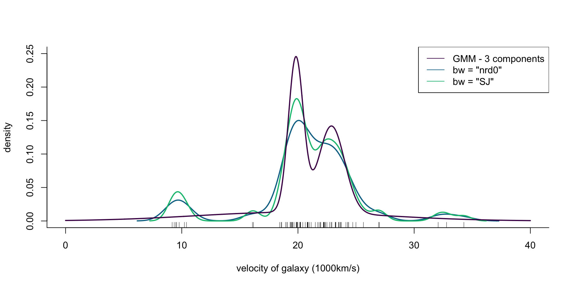
Figure 4: Density of galaxy velocities in 1000km/s, using two kernel density estimators with gaussian kernel but different bandwidth selection procedures, and a mixture of 3 normal densities.
Velocity of galaxies: Model selection for density estimation
R code
plot(x = c(0, 40), y = c(0, 0.25), type = "n", bty = "l",
     xlab = "velocity of galaxy (1000km/s)", ylab = "density")
rug(galaxies)
lines(density(galaxies, bw = "nrd0"), col = cols[2], lwd = 2)
lines(density(galaxies, bw = "SJ"), col = cols[3], lwd = 2)
legend("topright", legend = c('GMM - 4 components', 'bw = "nrd0"', 'bw = "SJ"'),
       col = cols, lty = 1)
ra <- seq(0, 40, length.out = 1000)
gal_mix <- Mclust(galaxies, G = 4, modelNames = "V")
lines(ra, dens(ra, modelName = "V", parameters = gal_mix$parameters),
      col = cols[1], lwd = 2)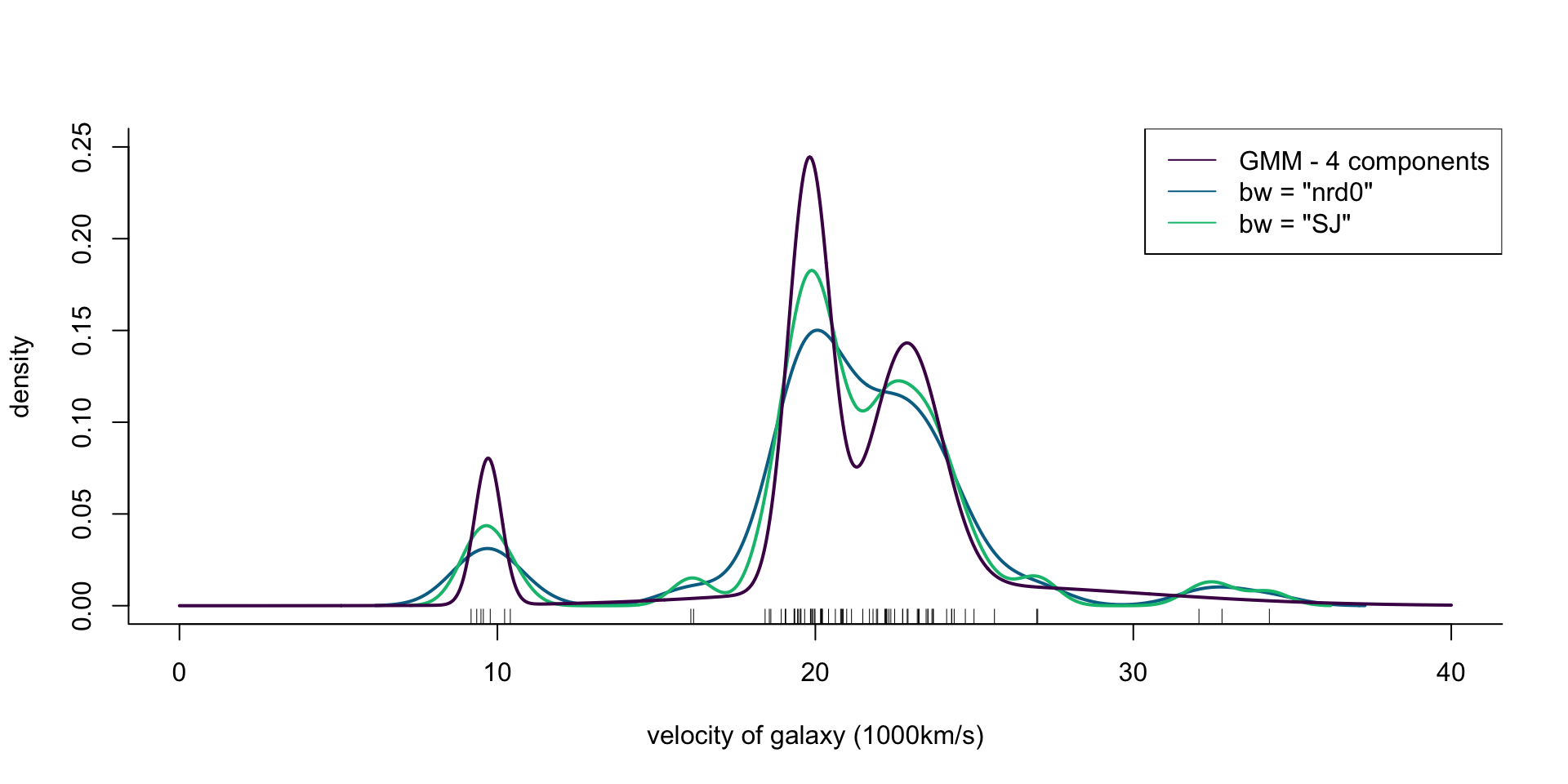
Figure 5: Density of galaxy velocities in 1000km/s, using two kernel density estimators with gaussian kernel but different bandwidth selection procedures, and a mixture of 4 normal densities.
Velocity of galaxies: Model selection for density estimation
R code
plot(x = c(0, 40), y = c(0, 0.25), type = "n", bty = "l",
     xlab = "velocity of galaxy (1000km/s)", ylab = "density")
rug(galaxies)
lines(density(galaxies, bw = "nrd0"), col = cols[2], lwd = 2)
lines(density(galaxies, bw = "SJ"), col = cols[3], lwd = 2)
legend("topright", legend = c('GMM - 5 components', 'bw = "nrd0"', 'bw = "SJ"'),
       col = cols, lty = 1)
ra <- seq(0, 40, length.out = 1000)
gal_mix <- Mclust(galaxies, G = 5, modelNames = "V")
lines(ra, dens(ra, modelName = "V", parameters = gal_mix$parameters),
      col = cols[1], lwd = 2)
Figure 6: Density of galaxy velocities in 1000km/s, using two kernel density estimators with gaussian kernel but different bandwidth selection procedures, and a mixture of 5 normal densities.
Velocity of galaxies: Model selection for density estimation
R code
plot(x = c(0, 40), y = c(0, 0.25), type = "n", bty = "l",
     xlab = "velocity of galaxy (1000km/s)", ylab = "density")
rug(galaxies)
lines(density(galaxies, bw = "nrd0"), col = cols[2], lwd = 2)
lines(density(galaxies, bw = "SJ"), col = cols[3], lwd = 2)
legend("topright", legend = c('GMM - 6 components', 'bw = "nrd0"', 'bw = "SJ"'),
       col = cols, lty = 1)
ra <- seq(0, 40, length.out = 1000)
gal_mix <- Mclust(galaxies, G = 6, modelNames = "V")
lines(ra, dens(ra, modelName = "V", parameters = gal_mix$parameters),
      col = cols[1], lwd = 2)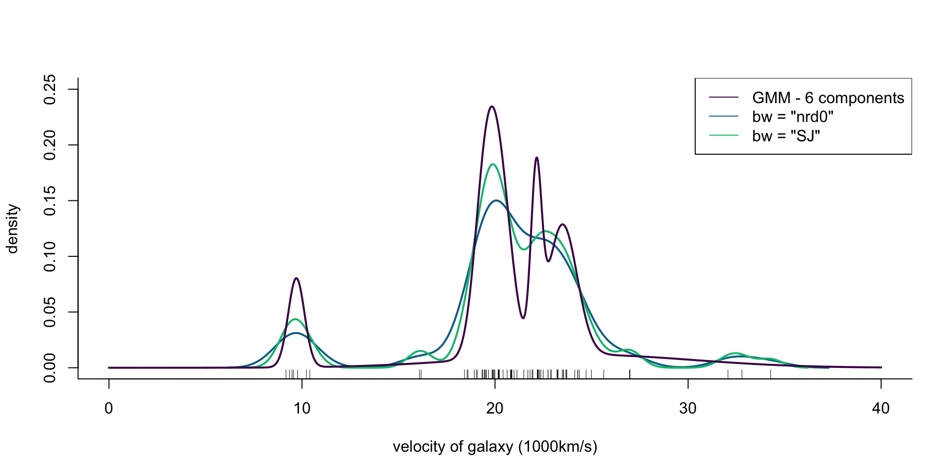
Figure 7: Density of galaxy velocities in 1000km/s, using two kernel density estimators with gaussian kernel but different bandwidth selection procedures, and a mixture of 6 normal densities.
Velocity of galaxies: Model selection for density estimation
R code
plot(x = c(0, 40), y = c(0, 0.25), type = "n", bty = "l",
     xlab = "velocity of galaxy (1000km/s)", ylab = "density")
rug(galaxies)
lines(density(galaxies, bw = "nrd0"), col = cols[2], lwd = 2)
lines(density(galaxies, bw = "SJ"), col = cols[3], lwd = 2)
legend("topright", legend = c('GMM - 7 components', 'bw = "nrd0"', 'bw = "SJ"'),
       col = cols, lty = 1)
ra <- seq(0, 40, length.out = 1000)
gal_mix <- Mclust(galaxies, G = 7, modelNames = "V")
lines(ra, dens(ra, modelName = "V", parameters = gal_mix$parameters),
      col = cols[1], lwd = 2)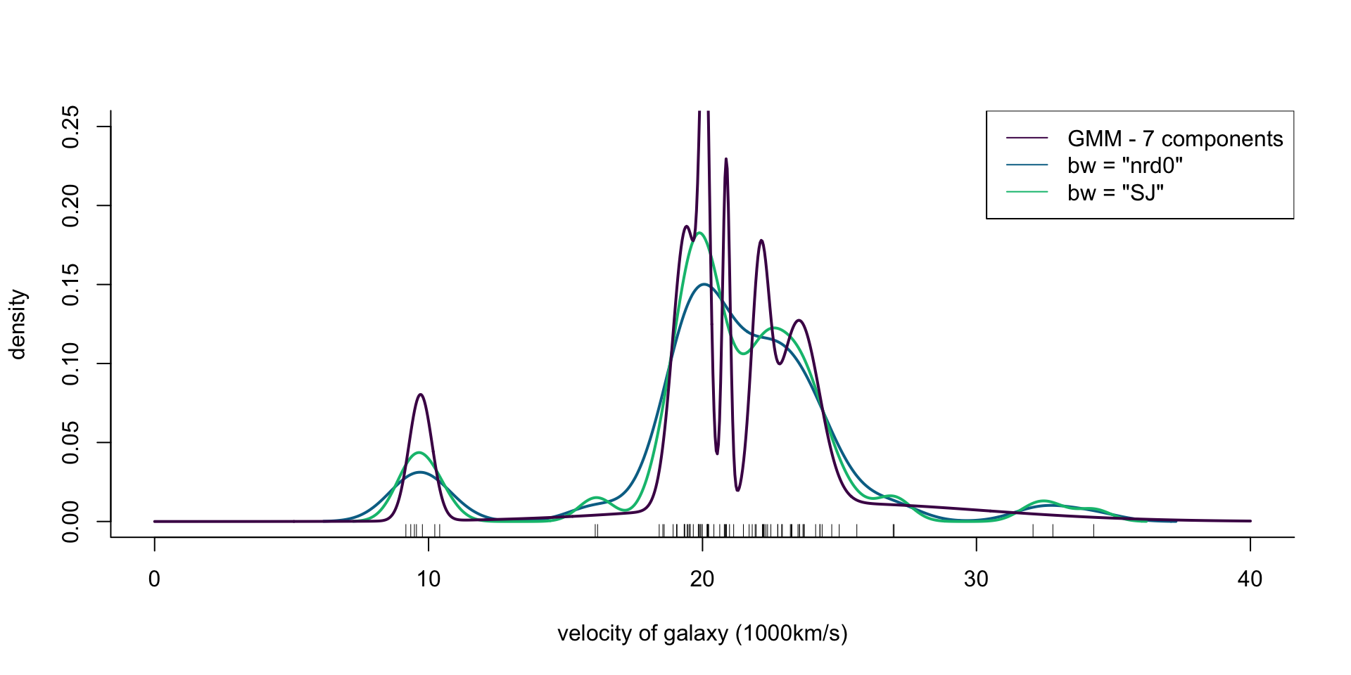
Figure 8: Density of galaxy velocities in 1000km/s, using two kernel density estimators with gaussian kernel but different bandwidth selection procedures, and a mixture of 7 normal densities.
Principles: Models are approximations
Remember that all models are wrong; the practical question is how wrong do they have to be to not be useful. 1
Typically, there is no “correct” or “true” model, and even if there is one, it is often unknown and/or very complex. Of most practical value is to find and work with a simple model that performs well in some sense.
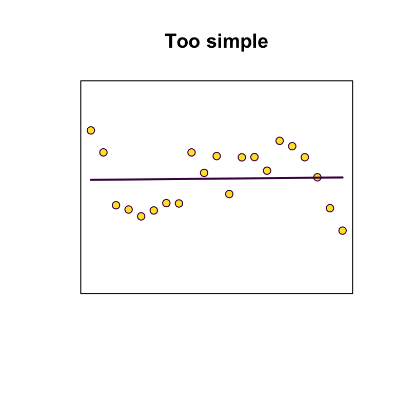
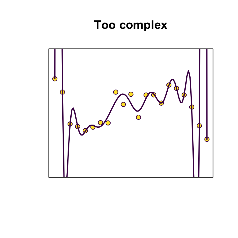
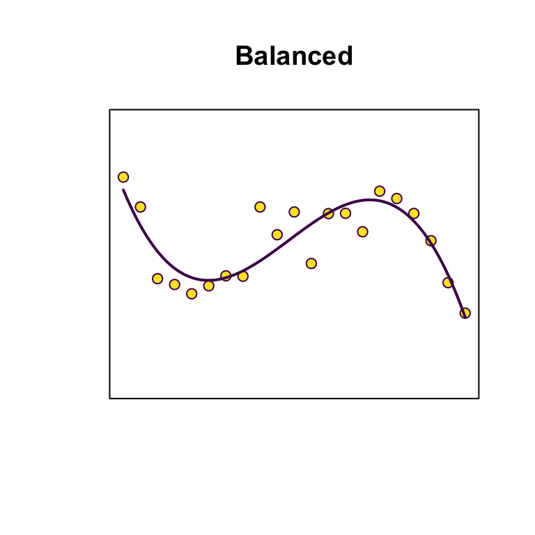
Principles: Bias-variance trade-off
Strike a balance between overfitting (too many parameters, model is unlikely to perform well out-of-sample) and underfitting (too few parameters, not capturing sufficient signal).
| Bias | Variance | |
|---|---|---|
| Simplicity | higher | lower |
| Complexity | lower | higher |
Principles: Parsimony

Entities should not be multiplied beyond necessity.
Only parameters that really matter for the particular aims of the analysis ought to be included in a selected model.
Principles: Context and focus

How odd it is that anyone should not see that all observation must be for or against some view if it is to be of any service.
All modelling is rooted in a specific scientific context and serves a particular purpose.
Different researchers may interpret the same data differently, and different scientific schools may have varying preferences for modelling and data analysis aims.
The purpose of models can vary, ranging from prediction and classification to deeper understanding of the underlying model1 to learning specific quantities well.
Principles for candidate sets of models in variable selection
Principle of marginality
Unless substantive knowledge dictates otherwise,
If an interaction is present, then keep all respective main effects.
If a higher-order term is present (e.g. \(x^3\)), then keep all lower-order terms (e.g. \(x\) and \(x^2\)).
Keep the intercept parameter in.
1, 3 are essential for explanatory modelling, and all 1-3 avoid some very specific models. e.g.
R code
set.seed(123)
x <- seq(-10, 10, length.out = 100)
y <-  10 + 3 * x + 0.25 * x^2 + rnorm(100, 0, 10)
forms <- c(y ~ x, y ~ x + I(x^2), y ~ I(x^2), y ~ -1 + x, y ~ -1 + x + I(x^2), y ~ -1 + I(x^2))
df <- NULL
for (f in forms) {
    df <- rbind(df, data.frame(x = x, y = y, yhat = predict(lm(f)), model = deparse(f)))
}
df <- df |> transform(model = factor(model, levels = sapply(forms, deparse), ordered = TRUE))
ggplot(df) +
    geom_point(aes(x, y), pch = 21, fill = cols[4]) +
    geom_line(aes(x, yhat), size = 1, col = cols[1]) +
    facet_grid(~ model) +
    theme_minimal() +
    theme(legend.position = "none", axis.ticks = NULL)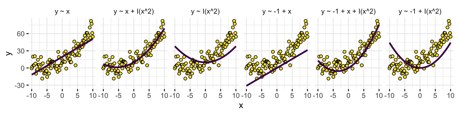
Nodal involvement
Considering only the models with an intercept and without any interaction between the 5 binary covariates, results in \(2^5 = 32\) possible logistic regression models for this data.
R code

Figure 9: Maximized log-likelihoods for 32 possible logistic regression models for the nodal data.
Adding terms always increases the maximized log-likelihood.
Simply, taking the model with highest \(\hat\ell\) would give the model with all parameters.
Polynomial regression
\(n = 20\)
R code
Delta <- function(p, p0, x, sigma2) {
    cols <- 0:(p - 1)
    cols0 <- 0:(p0 - 1)
    n <- length(x)
    X <- matrix(rep(x, p)^rep(cols, each = n), nrow = n)
    X0 <- matrix(rep(x, p0)^rep(cols0, each = n), nrow = n)
    mu <- rowSums(X0)
    H <- tcrossprod(qr.Q(qr(X)))
    bias <- sum(((diag(n) - H) %*% mu)^2) / n
    variance <- sigma2 * (1 + p / n)
    c(p = p, bias = bias, variance = variance)
}

n <- 20
sigma2 <- 2
p_max <- 15
p0 <- 6
set.seed(1)
x <- rnorm(n)
D <- data.frame(t(sapply(1:p_max, Delta, p0 = p0, x = x, sigma2 = 1)))
par(mfrow = c(1, 3))
plot(bias ~ p, data = D, subset = p > 3,
     main = expression("Bias"^2), ylab = "",
     type = "b", bg = cols[1], pch = 21)
abline(v = p0, lty = 3, col = "grey")
plot(variance ~ p, data = D, subset = p > 3,
     main = expression("Variance"), ylab = "",
     type = "b", bg = cols[2], pch = 21)
abline(v = p0, lty = 3, col = "grey")
plot(bias + variance ~ p, data = D, subset = p > 3,
     main = expression(Delta), ylab = "",
     type = "b", bg = cols[3], pch = 21)
abline(v = p0, lty = 3, col = "grey")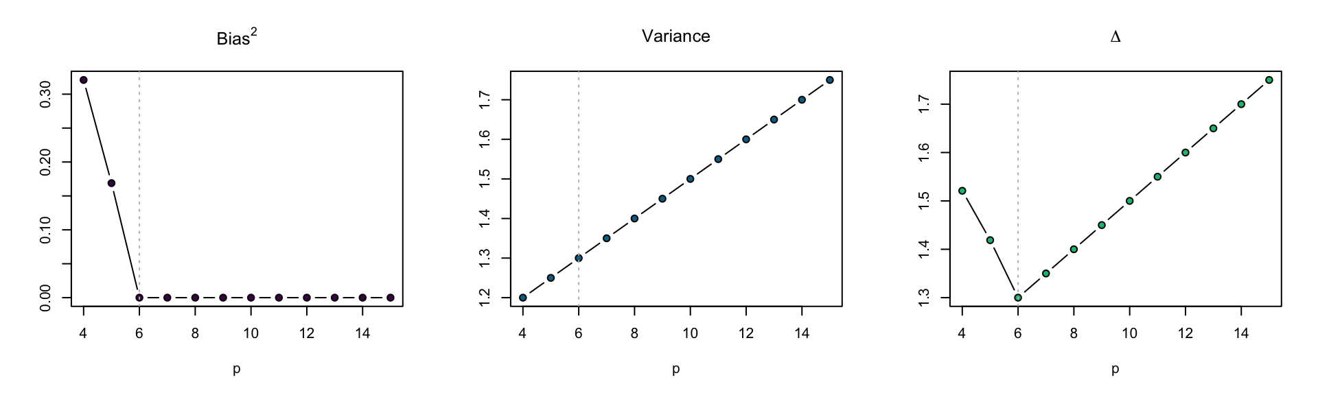
Figure 10: \(\Delta\) for models with varying polynomial degree.
Nodal involvement
Considering only the models with an intercept and without any interaction between the 5 binary covariates, results in \(2^5 = 32\) possible logistic regression models for this data.
R code
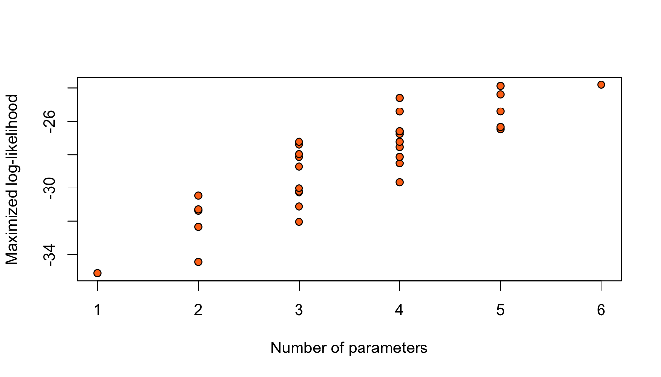
Figure 11: Maximized log-likelihoods for 32 possible logistic regression models for the nodal data.
Adding terms always increases the maximized log-likelihood.
Simply, taking the model with highest \(\hat\ell\) would give the model with all parameters.
\[ P(A \mid B) = \frac{P(B \mid A) P(A)}{P(B)} \]
in Bayes (1763/4). Essay towards solving a problem in the doctrine of chances. Philosophical Transactions of the Royal Society of London.

A joke by Xiao-Li Meng
Nodal involvement: AIC, BIC
R code
par(mfrow = c(1, 2))
plot(AIC ~ df, data = mods_AIC, xlab = "Number of parameters",
     bg = "#ff7518", pch = 21)
points(AIC ~ df, data = mods_AIC |> aggregate(AIC ~ df, min), type = "l")
plot(BIC ~ df, data = mods_BIC, xlab = "Number of parameters",
     bg = "#ff7518", pch = 21)
points(BIC ~ df, data = mods_BIC |> aggregate(BIC ~ df, min), type = "l")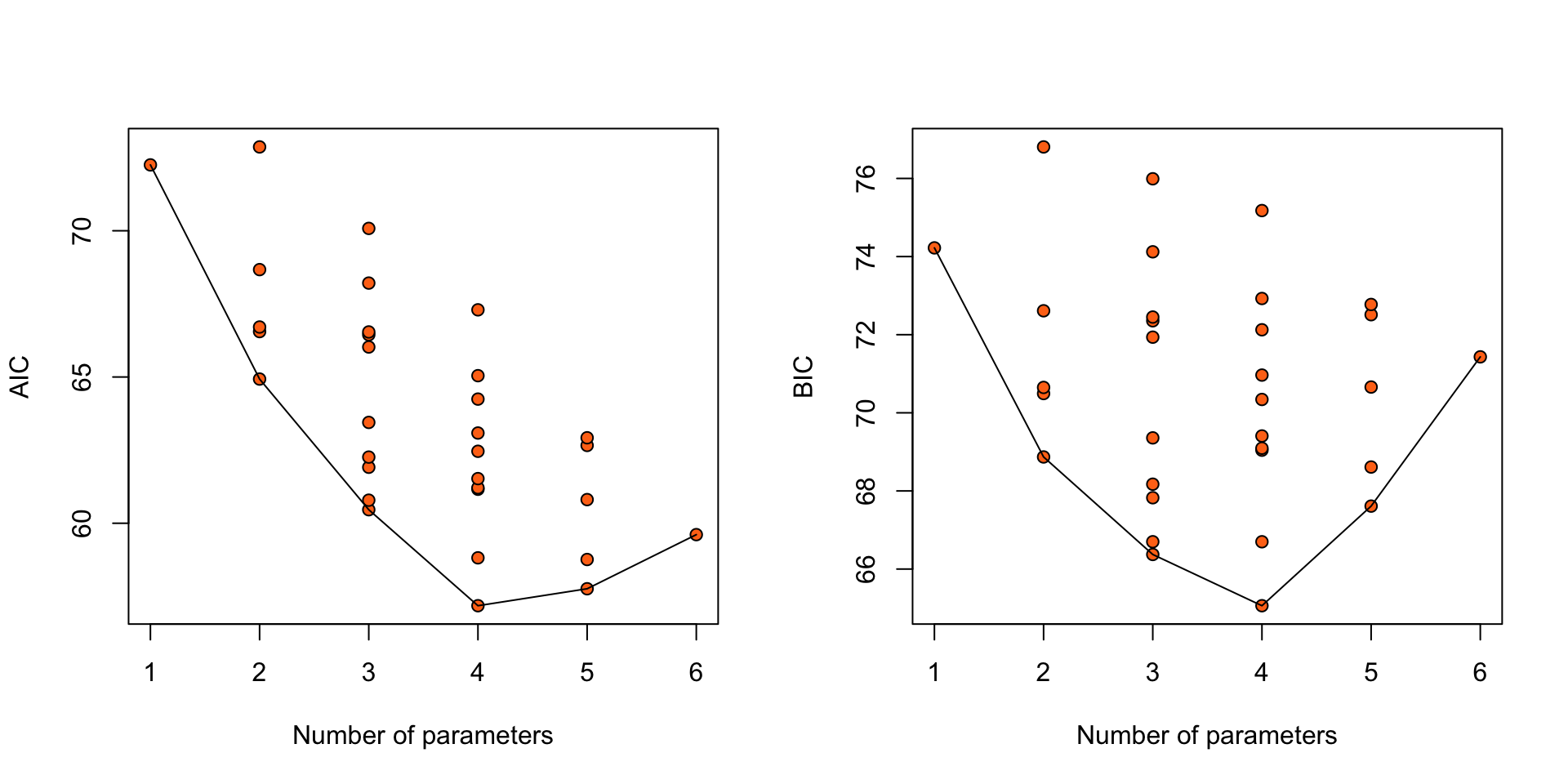
Figure 12: AIC and BIC for 32 logistic regression models for the nodal data.
Simulation study: Linear regression
\(\beta = (3, 2, 1, 1, 1, 1, 0)^\top\), \(\sigma = 1\)
R code
ns <- c(10, 20, 40, 80, 160, 320, 640)
set.seed(123)
sel_probs <- lapply(ns, function(n) selection_frequencies(1000, n, c(3, 2, 1, 1, 1, 1, 0)))
sel_probs <- do.call("rbind", sel_probs)
ggplot(sel_probs) +
    geom_col(aes(x = model, y = freq, color = IC, fill = IC), position = "dodge") +
    facet_grid(IC ~ n, labeller = label_both) +
    theme_minimal() +
    labs(x = "# of covariates", y = "Selection frequency")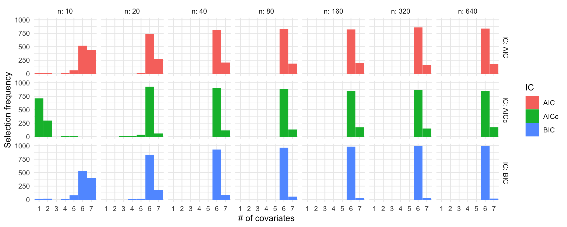
Simulation study: Linear regression
\(\beta = (3, 2, 1, 0, 0, 0, 0)^\top\), \(\sigma = 1\)
R code
ns <- c(10, 20, 40, 80, 160, 320, 640)
set.seed(123)
sel_probs <- lapply(ns, function(n) selection_frequencies(1000, n, c(3, 2, 1, 0, 0, 0, 0)))
sel_probs <- do.call("rbind", sel_probs)
ggplot(sel_probs) +
    geom_col(aes(x = model, y = freq, color = IC, fill = IC), position = "dodge") +
    facet_grid(IC ~ n, labeller = label_both) +
    theme_minimal() +
    labs(x = "# of covariates", y = "Selection frequency")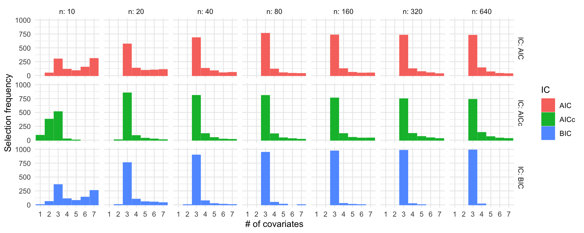
Simulation study: Linear regression
\(\beta = (3, 0, 0, 0, 0, 0, 0)^\top\), \(\sigma = 1\)
R code
ns <- c(10, 20, 40, 80, 160, 320, 640)
set.seed(123)
sel_probs <- lapply(ns, function(n) selection_frequencies(1000, n, c(3, 0, 0, 0, 0, 0, 0)))
sel_probs <- do.call("rbind", sel_probs)
ggplot(sel_probs) +
    geom_col(aes(x = model, y = freq, color = IC, fill = IC), position = "dodge") +
    facet_grid(IC ~ n, labeller = label_both) +
    theme_minimal() +
    labs(x = "# of covariates", y = "Selection frequency")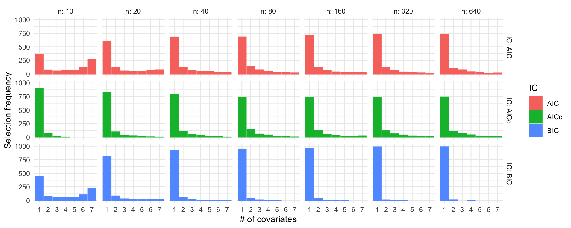
Simulation study: Linear regression
\(\beta = (3, 2, 1, 0, 0, 0, 0)^\top\), \(\sigma = 1\)
R code
ns <- c(10, 20, 40, 80, 160, 320, 640)
set.seed(123)
sel_probs <- lapply(ns, function(n) selection_frequencies(1000, n, c(3, 2, 1, 0, 0, 0, 0)))
sel_probs <- do.call("rbind", sel_probs)
ggplot(sel_probs) +
    geom_col(aes(x = model, y = freq, color = IC, fill = IC), position = "dodge") +
    facet_grid(IC ~ n, labeller = label_both) +
    theme_minimal() +
    labs(x = "# of covariates", y = "Selection frequency")
Simulation study: Linear regression
\(\beta = (3, 2, 1, 0, 0, 0, 0)^\top\), \(\sigma = 3\)
R code
ns <- c(10, 20, 40, 80, 160, 320, 640)
set.seed(123)
sel_probs <- lapply(ns, function(n) selection_frequencies(1000, n, c(3, 2, 1, 0, 0, 0, 0), sigma = 3))
sel_probs <- do.call("rbind", sel_probs)
ggplot(sel_probs) +
    geom_col(aes(x = model, y = freq, color = IC, fill = IC), position = "dodge") +
    facet_grid(IC ~ n, labeller = label_both) +
    theme_minimal() +
    labs(x = "# of covariates", y = "Selection frequency")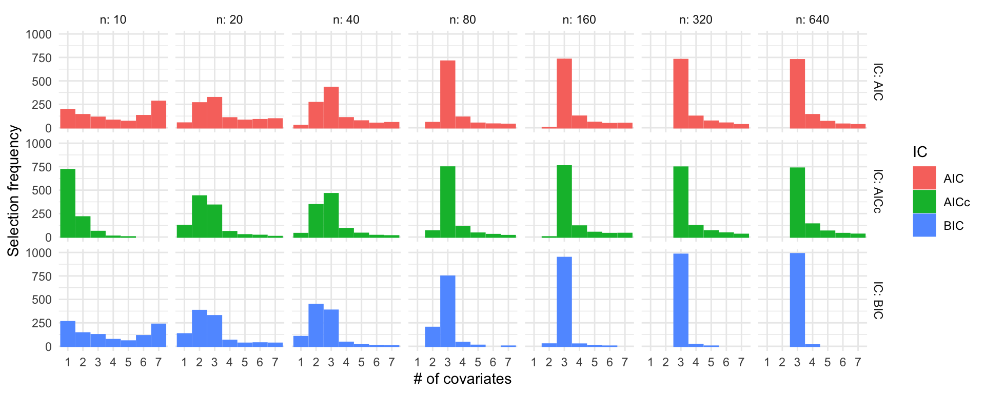
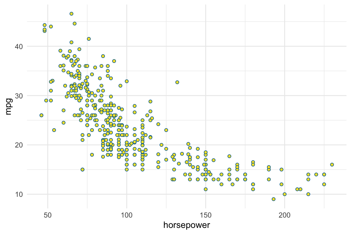
mpg ~ horsepower
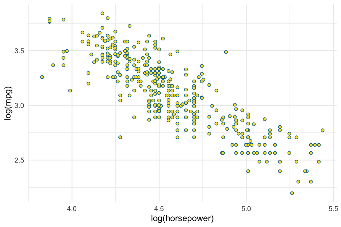
log(mpg) ~ log(horsepower)
Best \(m\) for mpg ~ poly(horsepower, m)
R code
cols0 <- hcl.colors(6, palette = "Dynamic")
ggplot(crits,
       aes(degree, value, col = criterion)) +
    geom_line() + geom_point() +
    theme_minimal() +
    labs(y = "criterion / min(criterion)") +
    lims(y = range(crits$value)) +
    scale_x_continuous(breaks = 1:10) +
    scale_color_manual(values = cols0) +
    facet_wrap(~ approach, scales = "free_y")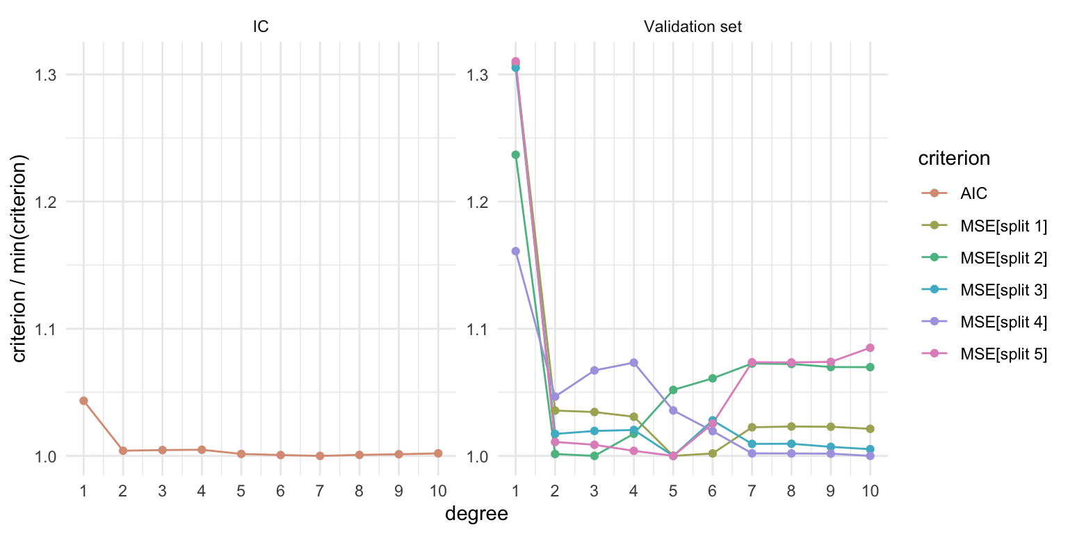
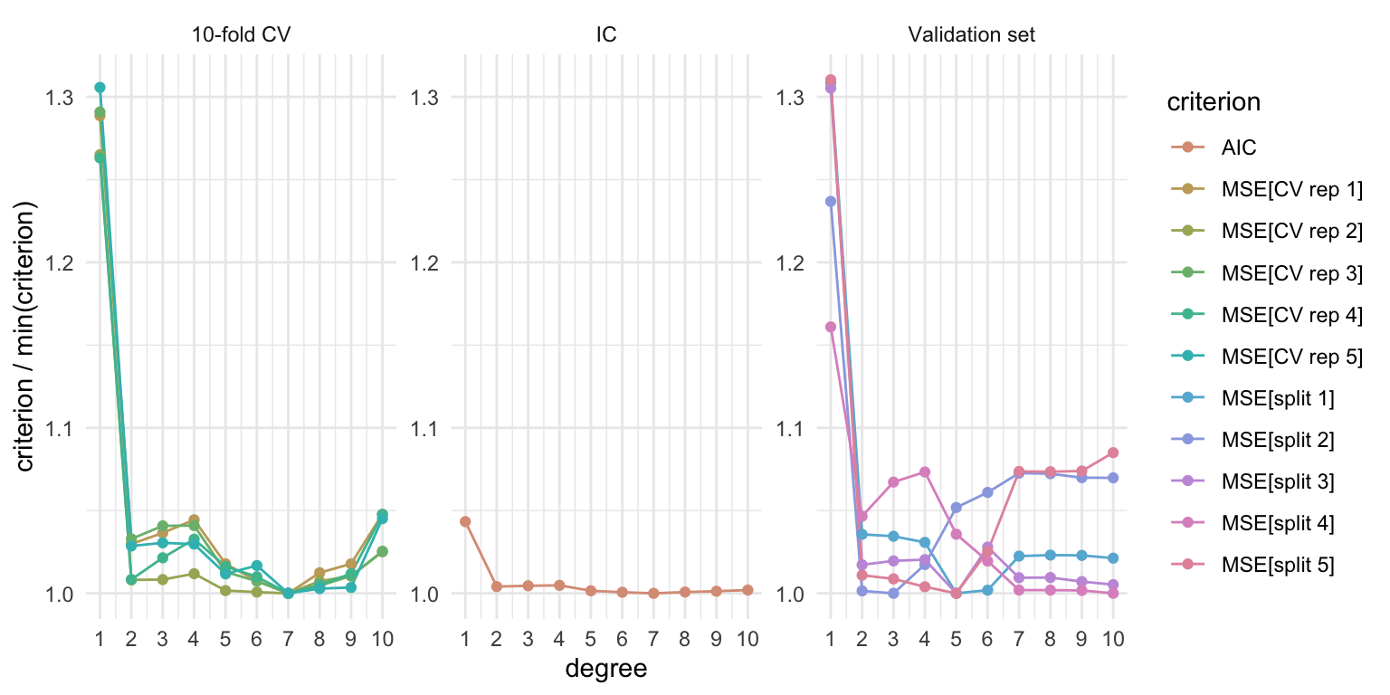
Best \(m\) for mpg ~ poly(horsepower, m)
R code
n_reps <- 5
n_folds <- 5
cvs <- replicate(n_reps, cv(models(mods), k = n_folds, data = Auto), simplify = FALSE)
MSEcv <- sapply(cvs, function(cvfit) sapply(cvfit, function(x) x[["CV crit"]]))

crits <- data.frame(degree = degrees,
                    criterion = rep(c(paste0("MSE[split ", 1:n_splits, "]"),
                                      paste0("MSE[CV rep ", 1:n_reps, "]"), "AIC"),
                                    each = length(degrees)),
                    approach = rep(c("Validation set", "10-fold CV", "IC"), c(n_splits * length(degrees), n_reps * length(degrees), length(degrees))),
                    value = c(c(MSEv), c(MSEcv), AICs), check.names = FALSE)
crits <- crits |> group_by(criterion) |> mutate(value = value / min(value))
cols0 <- hcl.colors(11, palette = "Dynamic")
ggplot(crits,
       aes(degree, value, col = criterion)) +
    geom_line() + geom_point() +
    theme_minimal() +
    labs(y = "criterion / min(criterion)") +
    lims(y = range(crits$value)) +
    scale_x_continuous(breaks = 1:10) +
    scale_color_manual(values = cols0) +
    facet_wrap(~ approach, scales = "free_y")